The purpose of this test is to show that there is correlation between modifiable argument in Vocaloid project file and quality of tuning.
What is Vocaloid? Here is a link to wiki page.
Vocaloid:
Vocaloid (ボーカロイド, Bōkaroido) is a singing voice synthesizer software product. Its signal processing part was developed through a joint research project led by Kenmochi Hideki at the Pompeu Fabra University in Barcelona, Spain, in 2000 and was not originally intended to be a full commercial project. Backed by the Yamaha Corporation, it developed the software into the commercial product “Vocaloid” which was released in 2004.
Project github repo: https://github.com/Discover304/AI-Tuner
Prepare dataset
In this part we will get a formated vsqx data in dictionary with 2 dimension infromation note and id.
- import vocaloid project (.vsqx) and extract all test related arguments (arg)
- format all args to 960 length list where 960 is the time stamps
1 | # adding path to system |
1. Thanks for the data from creator: 混音: リサRisa
	Source of data: https://www.vsqx.top/project/vn1801

2. Thanks for the data from creator: 扒谱:星葵/混音:seedking
	Source of data: https://www.vsqx.top/project/vn1743

3. Thanks for the data from creator: N/A
	Source of data: https://www.vsqx.top/project/vn1784

4. Thanks for the data from creator: vsqx:DZ韦元子
	Source of data: https://www.vsqx.top/project/vn1752

5. Thanks for the data from creator: N/A
	Source of data: https://www.vsqx.top/project/vn1749

6. Thanks for the data from creator: 填词~超监督乌鸦,千年食谱颂vsqx~的的的的的说,制作~cocok7
	Source of data: https://www.vsqx.top/project/vn1798

7. Thanks for the data from creator: 伴奏:小野道ono (https://www.dizzylab.net/albums/d/dlep02/)
	Source of data: https://www.vsqx.top/project/vn1788

8. Thanks for the data from creator: 调/混:邪云 扒谱:天啦噜我的串串儿
	Source of data: https://www.vsqx.top/project/vn1796

9. Thanks for the data from creator: 扒谱:磷元素P
	Source of data: https://www.vsqx.top/project/vn1753

10. Thanks for the data from creator: N/A
	Source of data: https://www.vsqx.top/project/vn1778
1 | # resolve all original data in parallel way, and save them to loacl |
It may take a while if the file are resolved for the first time.
local computer has: 16 cores

Parallal computing takes 0.00 seconds to finish.
1 | # load saved data |
Log: loaded
Log: loaded
Log: loaded
Log: loaded
Log: loaded
Log: loaded
Log: loaded
Log: loaded
Log: loaded
Log: loaded
| index | D | G | W | P | S | VEL | T | OPE | DUR | |
|---|---|---|---|---|---|---|---|---|---|---|
| 0 | 0 | [0, 0, 0, 0, 0, 0, 0, 0, 0, 0, 0, 0, 0, 0, 0, ... | [0, 0, 0, 0, 0, 0, 0, 0, 0, 0, 0, 0, 0, 0, 0, ... | [0, 0, 0, 0, 0, 0, 0, 0, 0, 0, 0, 0, 0, 0, 0, ... | [0, 0, 0, 0, 0, 0, 0, 0, 0, 0, 0, 0, 0, 0, 0, ... | [0, 0, 0, 0, 0, 0, 0, 0, 0, 0, 0, 0, 0, 0, 0, ... | [64, 64, 64, 64, 64, 64, 64, 64, 64, 64, 64, 6... | [0, 1, 2, 3, 4, 5, 6, 7, 8, 9, 10, 11, 12, 13,... | [127, 127, 127, 127, 127, 127, 127, 127, 127, ... | [90, 90, 90, 90, 90, 90, 90, 90, 90, 90, 90, 9... |
| 1 | 1 | [0, 0, 0, 0, 0, 0, 0, 0, 0, 0, 0, 0, 0, 0, 0, ... | [0, 0, 0, 0, 0, 0, 0, 0, 0, 0, 0, 0, 0, 0, 0, ... | [0, 0, 0, 0, 0, 0, 0, 0, 0, 0, 0, 0, 0, 0, 0, ... | [0, 0, 0, 0, 0, 0, 0, 0, 0, 0, 0, 0, 0, 0, 0, ... | [0, 0, 0, 0, 0, 0, 0, 0, 0, 0, 0, 0, 0, 0, 0, ... | [64, 64, 64, 64, 64, 64, 64, 64, 64, 64, 64, 6... | [0, 1, 2, 3, 4, 5, 6, 7, 8, 9, 10, 11, 12, 13,... | [127, 127, 127, 127, 127, 127, 127, 127, 127, ... | [30, 30, 30, 30, 30, 30, 30, 30, 30, 30, 30, 3... |
| 2 | 2 | [64, 64, 64, 64, 64, 64, 64, 64, 64, 64, 64, 6... | [0, 0, 0, 0, 0, 0, 0, 0, 0, 0, 0, 0, 0, 0, 0, ... | [0, 0, 0, 0, 0, 0, 0, 0, 0, 0, 0, 0, 0, 0, 0, ... | [2418, 2418, 2418, 2418, 2418, 2418, 2418, 241... | [0, 0, 0, 0, 0, 0, 0, 0, 0, 0, 0, 0, 0, 0, 0, ... | [64, 64, 64, 64, 64, 64, 64, 64, 64, 64, 64, 6... | [0, 1, 2, 3, 4, 5, 6, 7, 8, 9, 10, 11, 12, 13,... | [127, 127, 127, 127, 127, 127, 127, 127, 127, ... | [150, 150, 150, 150, 150, 150, 150, 150, 150, ... |
| 3 | 3 | [0, 0, 0, 0, 0, 0, 0, 0, 0, 0, 0, 0, 0, 0, 0, ... | [0, 0, 0, 0, 0, 0, 0, 0, 0, 0, 0, 0, 0, 0, 0, ... | [0, 0, 0, 0, 0, 0, 0, 0, 0, 0, 0, 0, 0, 0, 0, ... | [0, 0, 0, 0, 0, 0, 0, 0, 0, 0, 0, 0, 0, 0, 0, ... | [0, 0, 0, 0, 0, 0, 0, 0, 0, 0, 0, 0, 0, 0, 0, ... | [64, 64, 64, 64, 64, 64, 64, 64, 64, 64, 64, 6... | [0, 1, 2, 3, 4, 5, 6, 7, 8, 9, 10, 11, 12, 13,... | [127, 127, 127, 127, 127, 127, 127, 127, 127, ... | [30, 30, 30, 30, 30, 30, 30, 30, 30, 30, 30, 3... |
| 4 | 4 | [55, 55, 55, 55, 55, 55, 55, 55, 55, 55, 55, 5... | [0, 0, 0, 0, 0, 0, 0, 0, 0, 0, 0, 0, 0, 0, 0, ... | [0, 0, 0, 0, 0, 0, 0, 0, 0, 0, 0, 0, 0, 0, 0, ... | [0, 0, 0, 0, 0, 0, 0, 0, 0, 0, 0, 0, 0, 0, 0, ... | [0, 0, 0, 0, 0, 0, 0, 0, 0, 0, 0, 0, 0, 0, 0, ... | [64, 64, 64, 64, 64, 64, 64, 64, 64, 64, 64, 6... | [0, 1, 2, 3, 4, 5, 6, 7, 8, 9, 10, 11, 12, 13,... | [127, 127, 127, 127, 127, 127, 127, 127, 127, ... | [30, 30, 30, 30, 30, 30, 30, 30, 30, 30, 30, 3... |
1 | 2248*9*960 |
19422720
Formating data before evaluation
The above dataframe is scary, with 19 million data as 3 dimension. We have to reduce the data by extract the main features of each 960 vector, and join to a dataframe. So, the next challenge we face is how to extract this features.
We decide to take following data:
- Continuous: VEL OPE DUR
- Discrete: D G W P S
- fearure without 0s:
- mid, mean, sd, mod
Continuousmeans one note one value,Discretemeans one time stamp one value
See more: https://www.cnblogs.com/xingshansi/p/6815217.html
1 | def zcr(dataArray): |
1 | # get discrete args fearure |
| VEL-SINGLE | OPE-SINGLE | DUR-SINGLE | |
|---|---|---|---|
| 0 | 64 | 127 | 90 |
| 1 | 64 | 127 | 30 |
| 2 | 64 | 127 | 150 |
| 3 | 64 | 127 | 30 |
| 4 | 64 | 127 | 30 |
1 | # get continuous args feature |
| D-MEAN | G-MEAN | W-MEAN | P-MEAN | S-MEAN | D-MID | G-MID | W-MID | P-MID | S-MID | D-SD | G-SD | W-SD | P-SD | S-SD | D-MOD | G-MOD | W-MOD | P-MOD | S-MOD | |
|---|---|---|---|---|---|---|---|---|---|---|---|---|---|---|---|---|---|---|---|---|
| 0 | 0.000000 | 0.0 | 0.0 | 0.000000 | 0.0 | 0.0 | 0.0 | 0.0 | 0.0 | 0.0 | 0.000000 | 0.0 | 0.0 | 0.000000 | 0.0 | 0 | 0 | 0 | 0 | 0 |
| 1 | 0.000000 | 0.0 | 0.0 | 0.000000 | 0.0 | 0.0 | 0.0 | 0.0 | 0.0 | 0.0 | 0.000000 | 0.0 | 0.0 | 0.000000 | 0.0 | 0 | 0 | 0 | 0 | 0 |
| 2 | 63.576159 | 0.0 | 0.0 | 2401.986755 | 0.0 | 64.0 | 0.0 | 0.0 | 2418.0 | 0.0 | 5.190972 | 0.0 | 0.0 | 196.121397 | 0.0 | 64 | 0 | 0 | 2418 | 0 |
| 3 | 0.000000 | 0.0 | 0.0 | 0.000000 | 0.0 | 0.0 | 0.0 | 0.0 | 0.0 | 0.0 | 0.000000 | 0.0 | 0.0 | 0.000000 | 0.0 | 0 | 0 | 0 | 0 | 0 |
| 4 | 53.225806 | 0.0 | 0.0 | 0.000000 | 0.0 | 55.0 | 0.0 | 0.0 | 0.0 | 0.0 | 9.717658 | 0.0 | 0.0 | 0.000000 | 0.0 | 55 | 0 | 0 | 0 | 0 |
1 | # join both discrete and continuous args dataframe |
| VEL-SINGLE | OPE-SINGLE | DUR-SINGLE | D-MEAN | G-MEAN | W-MEAN | P-MEAN | S-MEAN | D-MID | G-MID | ... | D-SD | G-SD | W-SD | P-SD | S-SD | D-MOD | G-MOD | W-MOD | P-MOD | S-MOD | |
|---|---|---|---|---|---|---|---|---|---|---|---|---|---|---|---|---|---|---|---|---|---|
| 0 | 64 | 127 | 90 | 0.000000 | 0.0 | 0.0 | 0.000000 | 0.0 | 0.0 | 0.0 | ... | 0.000000 | 0.0 | 0.0 | 0.000000 | 0.0 | 0 | 0 | 0 | 0 | 0 |
| 1 | 64 | 127 | 30 | 0.000000 | 0.0 | 0.0 | 0.000000 | 0.0 | 0.0 | 0.0 | ... | 0.000000 | 0.0 | 0.0 | 0.000000 | 0.0 | 0 | 0 | 0 | 0 | 0 |
| 2 | 64 | 127 | 150 | 63.576159 | 0.0 | 0.0 | 2401.986755 | 0.0 | 64.0 | 0.0 | ... | 5.190972 | 0.0 | 0.0 | 196.121397 | 0.0 | 64 | 0 | 0 | 2418 | 0 |
| 3 | 64 | 127 | 30 | 0.000000 | 0.0 | 0.0 | 0.000000 | 0.0 | 0.0 | 0.0 | ... | 0.000000 | 0.0 | 0.0 | 0.000000 | 0.0 | 0 | 0 | 0 | 0 | 0 |
| 4 | 64 | 127 | 30 | 53.225806 | 0.0 | 0.0 | 0.000000 | 0.0 | 55.0 | 0.0 | ... | 9.717658 | 0.0 | 0.0 | 0.000000 | 0.0 | 55 | 0 | 0 | 0 | 0 |
5 rows × 23 columns
1 | # get the rank list from our data list file (we has already import as json) |
| RANK | |
|---|---|
| 0 | 6 |
| 1 | 6 |
| 2 | 6 |
| 3 | 6 |
| 4 | 6 |
1 | # join our args rank dataframe together |
| VEL-SINGLE | OPE-SINGLE | DUR-SINGLE | D-MEAN | G-MEAN | W-MEAN | P-MEAN | S-MEAN | D-MID | G-MID | ... | G-SD | W-SD | P-SD | S-SD | D-MOD | G-MOD | W-MOD | P-MOD | S-MOD | RANK | |
|---|---|---|---|---|---|---|---|---|---|---|---|---|---|---|---|---|---|---|---|---|---|
| 0 | 64 | 127 | 90 | 0.000000 | 0.0 | 0.0 | 0.000000 | 0.0 | 0.0 | 0.0 | ... | 0.0 | 0.0 | 0.000000 | 0.0 | 0 | 0 | 0 | 0 | 0 | 6 |
| 1 | 64 | 127 | 30 | 0.000000 | 0.0 | 0.0 | 0.000000 | 0.0 | 0.0 | 0.0 | ... | 0.0 | 0.0 | 0.000000 | 0.0 | 0 | 0 | 0 | 0 | 0 | 6 |
| 2 | 64 | 127 | 150 | 63.576159 | 0.0 | 0.0 | 2401.986755 | 0.0 | 64.0 | 0.0 | ... | 0.0 | 0.0 | 196.121397 | 0.0 | 64 | 0 | 0 | 2418 | 0 | 6 |
| 3 | 64 | 127 | 30 | 0.000000 | 0.0 | 0.0 | 0.000000 | 0.0 | 0.0 | 0.0 | ... | 0.0 | 0.0 | 0.000000 | 0.0 | 0 | 0 | 0 | 0 | 0 | 6 |
| 4 | 64 | 127 | 30 | 53.225806 | 0.0 | 0.0 | 0.000000 | 0.0 | 55.0 | 0.0 | ... | 0.0 | 0.0 | 0.000000 | 0.0 | 55 | 0 | 0 | 0 | 0 | 6 |
5 rows × 24 columns
Clean our data
- delete all data that the dur longer than 1.5*IQR
- remove all 0 column
Notice: any other cleaning process should be done in this step
1 | l = np.quantile(dataDf['DUR-SINGLE'],0.25) |
1 | dataDf = dataDf[dataDf['DUR-SINGLE']<=IQR].reset_index() |
Observe data
Perform the following steps:
- normalise our dataset (we choose to use normaliser instead of standardiser, because there is a limit in the score which is about 100, it is more meaningful if we use normaliser)
- play with data to see if there are some observable trend of data
- plot the heat map of regression coefficient, and leave one argument from the pair with higher value
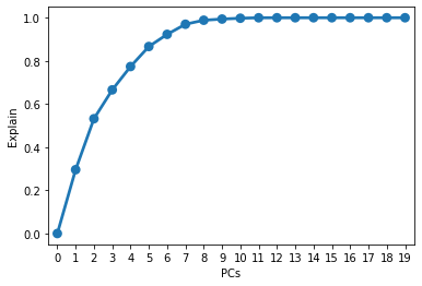
- fit to PCA modle, plot the corresponding percentage variance in a scree plot, combine the first several PCA
- regress the MSE of sound onto the combined PCA
If the MSE is reasonaly small, we can accept this result.
Normalisation and Standardization
1 | # define a normaliser |
| VEL-SINGLE | OPE-SINGLE | DUR-SINGLE | D-MEAN | G-MEAN | P-MEAN | S-MEAN | D-MID | G-MID | P-MID | S-MID | D-SD | G-SD | P-SD | S-SD | D-MOD | G-MOD | P-MOD | S-MOD | RANK | |
|---|---|---|---|---|---|---|---|---|---|---|---|---|---|---|---|---|---|---|---|---|
| 0 | 0.503937 | 1.0 | 0.198614 | 0.000000 | 0.0 | 0.500042 | 0.0 | 0.000000 | 0.0 | 0.499785 | 0.0 | 0.000000 | 0.0 | 0.000000 | 0.0 | 0.000000 | 0.0 | 0.499785 | 0.0 | 0.0 |
| 1 | 0.503937 | 1.0 | 0.060046 | 0.000000 | 0.0 | 0.500042 | 0.0 | 0.000000 | 0.0 | 0.499785 | 0.0 | 0.000000 | 0.0 | 0.000000 | 0.0 | 0.000000 | 0.0 | 0.499785 | 0.0 | 0.0 |
| 2 | 0.503937 | 1.0 | 0.337182 | 0.503959 | 0.0 | 0.648399 | 0.0 | 0.503937 | 0.0 | 0.648429 | 0.0 | 0.151537 | 0.0 | 0.083406 | 0.0 | 0.503937 | 0.0 | 0.648429 | 0.0 | 0.0 |
| 3 | 0.503937 | 1.0 | 0.060046 | 0.000000 | 0.0 | 0.500042 | 0.0 | 0.000000 | 0.0 | 0.499785 | 0.0 | 0.000000 | 0.0 | 0.000000 | 0.0 | 0.000000 | 0.0 | 0.499785 | 0.0 | 0.0 |
| 4 | 0.503937 | 1.0 | 0.060046 | 0.421914 | 0.0 | 0.500042 | 0.0 | 0.433071 | 0.0 | 0.499785 | 0.0 | 0.283683 | 0.0 | 0.000000 | 0.0 | 0.433071 | 0.0 | 0.499785 | 0.0 | 0.0 |
Starting observe data
1 | # prepare for evaluation tool |
1 | print(len(dataDfNormalized.columns)) |
20


Index(['VEL-SINGLE', 'OPE-SINGLE', 'DUR-SINGLE', 'D-MEAN', 'G-MEAN', 'P-MEAN',
       'S-MEAN', 'D-MID', 'G-MID', 'P-MID', 'S-MID', 'D-SD', 'G-SD', 'P-SD',
       'S-SD', 'D-MOD', 'G-MOD', 'P-MOD', 'S-MOD', 'RANK'],
      dtype='object')
1 | # distributionPlot('DUR-SINGLE','P-SD',"RANK",dataDfNormalized) |
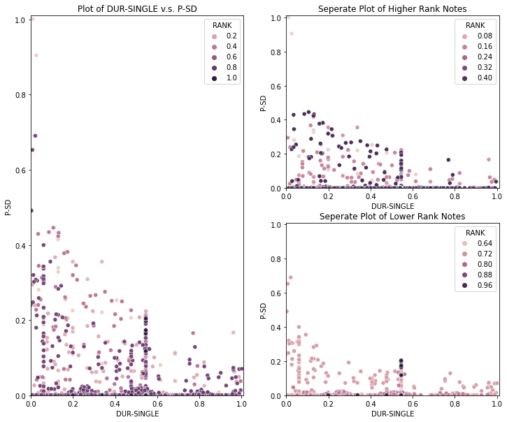
1 | tempDf = dataDfNormalized[dataDfNormalized['P-SD']!=0] |
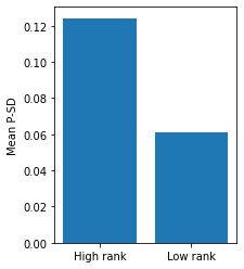
Observation 1
- The better the performance of a note in competition, the wider the pitch distributed and this trend can be seen along all duration value.
- A better tuner is more likly to change the pitch.
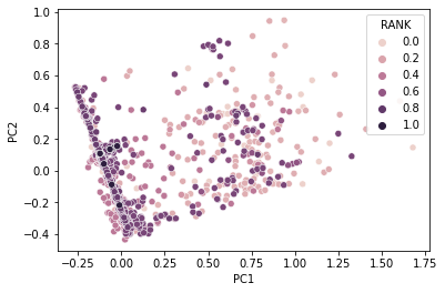
PCA
1 | dataDfNormalized.columns |
Index(['VEL-SINGLE', 'OPE-SINGLE', 'DUR-SINGLE', 'D-MEAN', 'G-MEAN', 'P-MEAN',
       'S-MEAN', 'D-MID', 'G-MID', 'P-MID', 'S-MID', 'D-SD', 'G-SD', 'P-SD',
       'S-SD', 'D-MOD', 'G-MOD', 'P-MOD', 'S-MOD', 'RANK'],
      dtype='object')
1 | from sklearn.decomposition import PCA |
1 | sns.pointplot(y = [np.sum(pca.explained_variance_ratio_[:i]) for i in range(20)], x = [i for i in range(20)]) |
linear regression
1 | import statsmodels.formula.api as smf |
| Dep. Variable: | RANK | R-squared: | 0.131 |
|---|---|---|---|
| Model: | OLS | Adj. R-squared: | 0.130 |
| Method: | Least Squares | F-statistic: | 106.3 |
| Date: | Mon, 11 Jan 2021 | Prob (F-statistic): | 1.68e-84 |
| Time: | 21:21:21 | Log-Likelihood: | 71.223 |
| No. Observations: | 2832 | AIC: | -132.4 |
| Df Residuals: | 2827 | BIC: | -102.7 |
| Df Model: | 4 | ||
| Covariance Type: | nonrobust |
| coef | std err | t | P>|t| | [0.025 | 0.975] | |
|---|---|---|---|---|---|---|
| Intercept | 0.5392 | 0.004 | 121.492 | 0.000 | 0.530 | 0.548 |
| PC1 | -0.3301 | 0.018 | -18.183 | 0.000 | -0.366 | -0.295 |
| PC2 | 0.1395 | 0.020 | 6.862 | 0.000 | 0.100 | 0.179 |
| PC3 | -0.1090 | 0.027 | -4.036 | 0.000 | -0.162 | -0.056 |
| PC4 | -0.1681 | 0.030 | -5.599 | 0.000 | -0.227 | -0.109 |
| Omnibus: | 28.744 | Durbin-Watson: | 0.186 |
|---|---|---|---|
| Prob(Omnibus): | 0.000 | Jarque-Bera (JB): | 19.880 |
| Skew: | -0.076 | Prob(JB): | 4.82e-05 |
| Kurtosis: | 2.619 | Cond. No. | 6.77 |
Notes:
[1] Standard Errors assume that the covariance matrix of the errors is correctly specified.
1 | pcs = pcs.join(pd.DataFrame({"RANK-PREDICT":result.fittedvalues}), on=pcs.index) |
1 | # the square error |
157.6792358196176
Visualise our regression result
1 | fig = plt.figure(figsize=(10,10)) |
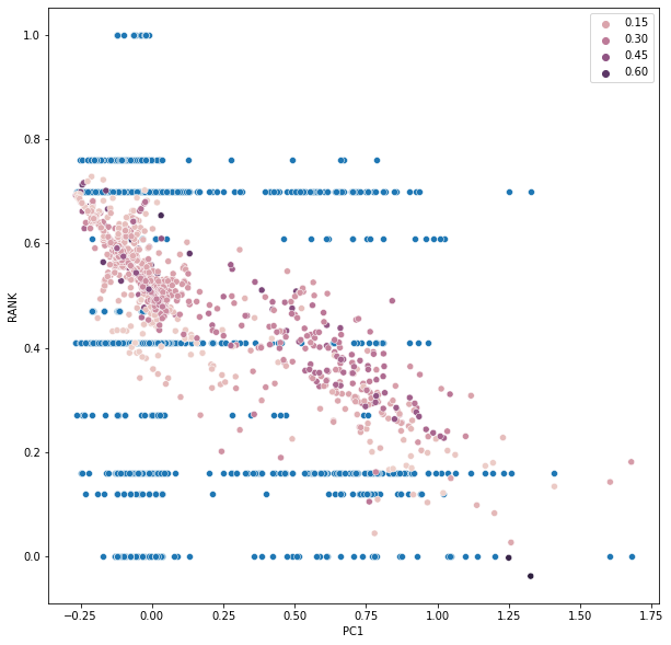
1 | fig = plt.figure(figsize=(10,10)) |
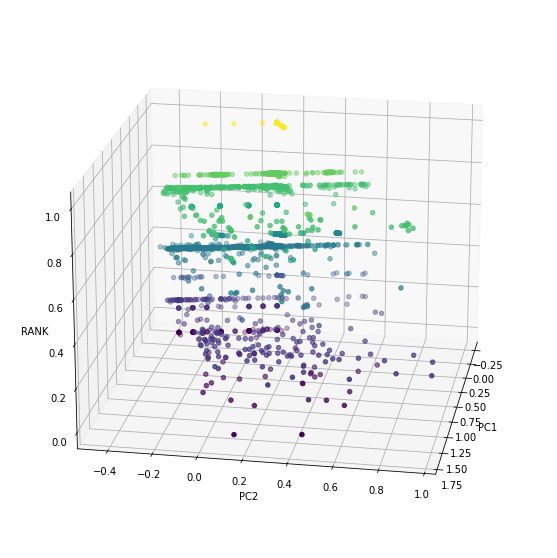
Conclusion
There is a really low value of $R^2$, less than 0.2, means the regression equation is not good enough to predict the Rank of a note from the properties we extracted from the 960 length vector. That might because of wrong choices of property, so, more research should be taken to varify the result we get in this notebook.
Next we can try to use the trend of a note to get a regression equation of it.