[toc]
OpenCV安装
执行以下命令安装opencv-python库(核心库)和opencv-contrib-python库(贡献库)。注意:命令拷贝后要合成一行执行,中间不要换行。
1 | 安装opencv核心库 |
OpenCV基本操作
读取、图像、保存图像
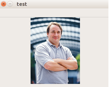
1 | # 读取图像 |
执行结果:
图像色彩操作
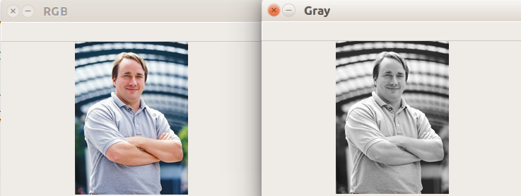
彩色图像转换为灰度图像
1 | # 彩色图像转换为灰度图像示例 |
执行结果:
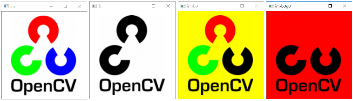
色彩通道操作
1 | # 色彩通道操作:通道表示为BGR |
执行结果:
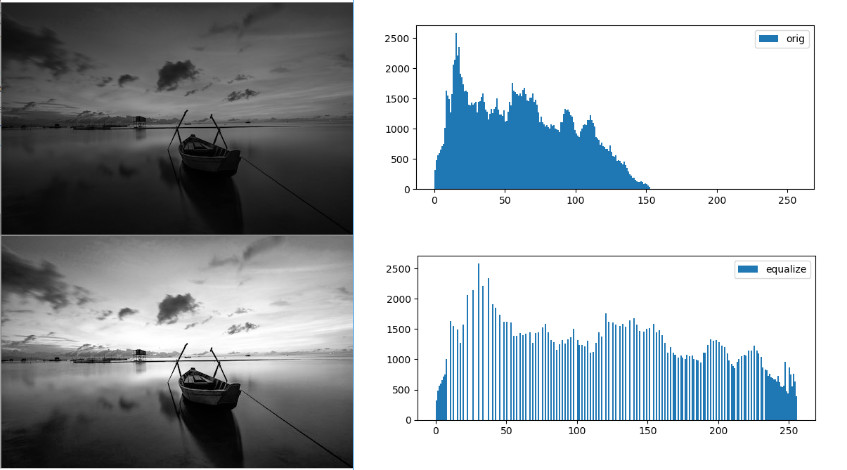
灰度直方图均衡化
1 | # 直方图均衡化示例 |
执行结果:
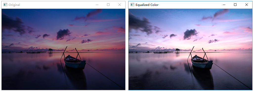
彩色亮度直方图均衡化
1 | # 彩色图像亮度直方图均衡化 |
执行结果:
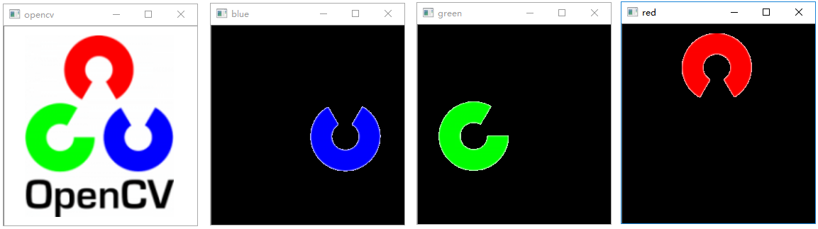
色彩提取
从图片中提取特定颜色
1 | import cv2 |
执行结果:
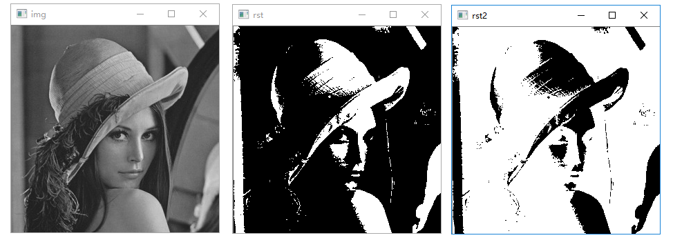
二值化与反二值化
1 | # 二值化处理 |
执行结果:
图像形态操作
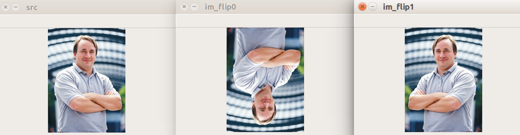
图像翻转
1 | # 图像翻转示例 |
执行结果:
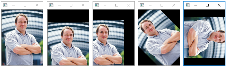
图像仿射变换
1 | # 图像仿射变换 |
执行结果:
图像缩放
1 | # 图像缩放示例 |
执行结果:

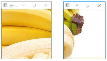
图像裁剪
1 | import numpy as np |
执行结果:
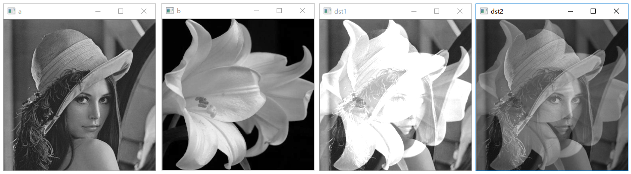
图像相加
1 | # 图像相加示例 |
执行结果:
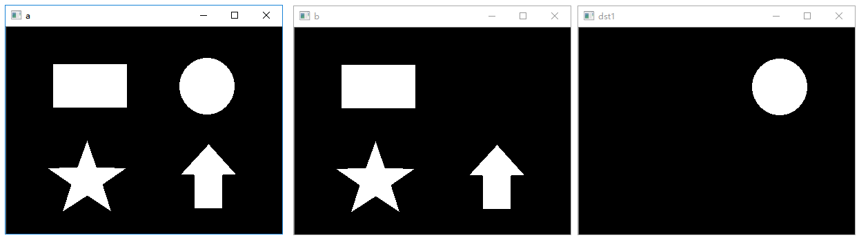
图像相减
1 | # 图像相减运算示例 |
执行结果:
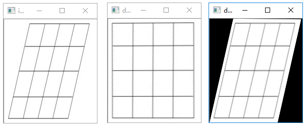
透视变换
1 | # 透视变换 |
执行结果:
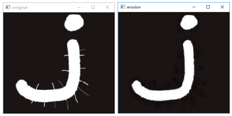
图像腐蚀
1 | # 图像腐蚀 |
执行结果:
图像膨胀
1 | # 图像膨胀 |
执行结果:
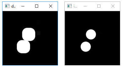
图像开运算
1 | # 开运算示例 |
执行结果:
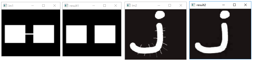
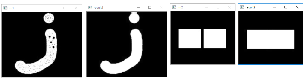
图像闭运算
1 | # 闭运算示例 |
执行结果:
形态学梯度
1 | # 形态学梯度示例 |
执行结果:

图像梯度处理
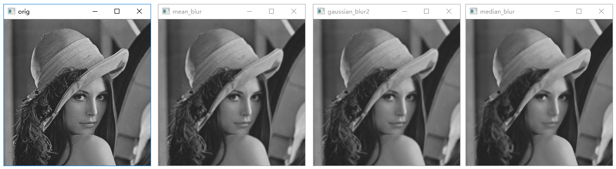
模糊处理
1 | # 图像模糊处理示例 |
执行结果:
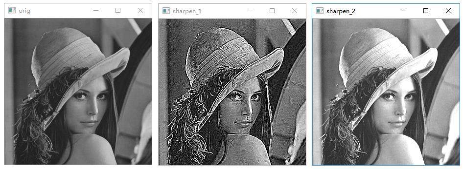
图像锐化处理
1 | # 图像锐化示例 |
执行结果:
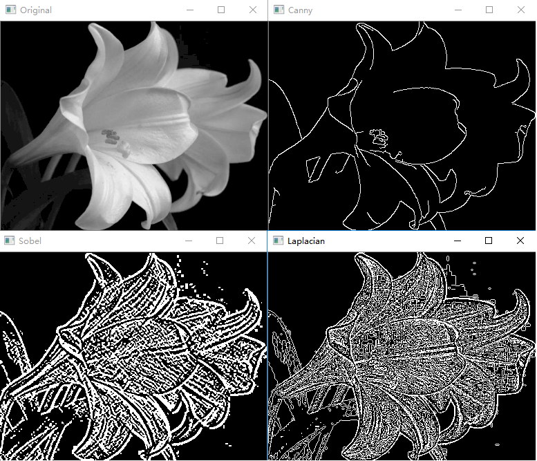
边沿检测
1 | # 边沿检测示例 |
执行结果:
轮廓处理
边缘检测虽然能够检测出边缘,但边缘是不连续的,检测到的边缘并不是一个整体。图像轮廓是指将边缘连接起来形成的一个整体,用于后续的计算。
OpenCV提供了查找图像轮廓的函数cv2.findContours(),该函数能够查找图像内的轮廓信息,而函数cv2.drawContours()能够将轮廓绘制出来。图像轮廓是图像中非常重要的一个特征信息,通过对图像轮廓的操作,我们能够获取目标图像的大小、位置、方向等信息。一个轮廓对应着一系列的点,这些点以某种方式表示图像中的一条曲线。
查找并绘制轮廓
-
查找轮廓函数:cv2.findContours
-
语法格式:image,contours,hierarchy=cv2.findContours(image,mode,method)
-
返回值
- image:与函数参数中的原始图像image一致
- contours:返回的轮廓。该返回值返回的是一组轮廓信息,每个轮廓都是由若干个点所构成的(每个轮廓为一个list表示)。例如,contours[i]是第i个轮廓(下标从0开始),contours[i][j]是第i个轮廓内的第j个点
- hierarchy:图像的拓扑信息(反映轮廓层次)。图像内的轮廓可能位于不同的位置。比如,一个轮廓在另一个轮廓的内部。在这种情况下,我们将外部的轮廓称为父轮廓,内部的轮廓称为子轮廓。按照上述关系分类,一幅图像中所有轮廓之间就建立了父子关系。每个轮廓contours[i]对应4个元素来说明当前轮廓的层次关系。其形式为:[Next,Previous,First_Child,Parent],分别表示后一个轮廓的索引编号、前一个轮廓的索引编号、第1个子轮廓的索引编号、父轮廓的索引编号
-
参数
- image:原始图像。灰度图像会被自动处理为二值图像。在实际操作时,可以根据需要,预先使用阈值处理等函数将待查找轮廓的图像处理为二值图像。
- mode:轮廓检索模式,有以下取值和含义:
取值 含义 cv2.RETR_EXTERNAL 只检测外轮廓 cv2.RETR_LIST 对检测到的轮廓不建立等级关系 cv2.RETR_CCOMP 检索所有轮廓并将它们组织成两级层次结构,上面的一层为外边界,下面的一层为内孔的边界 cv2.RETR_TREE 建立一个等级树结构的轮廓 - method:轮廓的近似方法,主要有如下取值:
取值 含义 cv2.CHAIN_APPROX_NONE 存储所有的轮廓点,相邻两个点的像素位置差不超过1,即max(abs(x1-x2),abs(y2-y1))=1 cv2.CHAIN_APPROX_SIMPLE 压缩水平方向、垂直方向、对角线方向的元素,只保留该方向的终点坐标 cv2.CHAIN_APPROX_TC89_L1 使用teh-Chinl chain近似算法的一种风格 cv2.CHAIN_APPROX_TC89_KCOS 使用teh-Chinl chain近似算法的一种风格 -
注意事项
- 待处理的源图像必须是灰度二值图
- 都是从黑色背景中查找白色对象。因此,对象必须是白色的,背景必须是黑色的
- 在OpenCV 4.x中,函数cv2.findContours()仅有两个返回值
-
-
绘制轮廓:drawContours函数
- 语法格式:image=cv2.drawContours(image, contours,contourIdx, color)
- 参数
- image:待绘制轮廓的图像
- contours:需要绘制的轮廓,该参数的类型与函数 cv2.findContours()的输出 contours 相同,都是list类型
- contourIdx:需要绘制的边缘索引,告诉函数cv2.drawContours()要绘制某一条轮廓还是全部轮廓。如果该参数是一个整数或者为零,则表示绘制对应索引号的轮廓;如果该值为负数(通常为“-1”),则表示绘制全部轮廓。
- color:绘制的颜色,用BGR格式表示
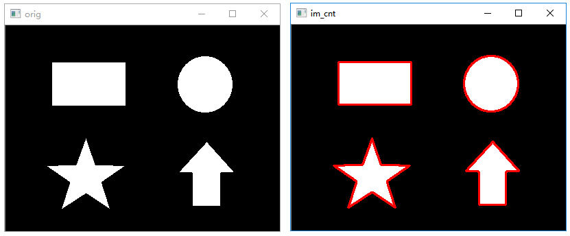
1 | # 查找图像轮廓 |
执行结果:
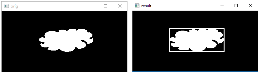
绘制矩形包围框
函数cv2.boundingRect()能够绘制轮廓的矩形边界。该函数的语法格式为:
1 | retval = cv2.boundingRect(array) # 格式一 |
代码:
1 | # 绘制图像矩形轮廓 |
执行结果:
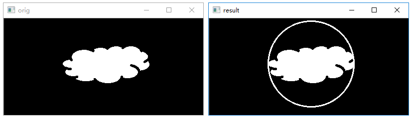
绘制圆形包围圈
函数 cv2.minEnclosingCircle()通过迭代算法构造一个对象的面积最小包围圆形。该函数的语法格式为:
1 | center,radius=cv2.minEnclosingCircle(points) |
代码:
1 | # 绘制最小圆形 |
执行结果:
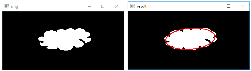
绘制最佳拟合椭圆
函数cv2.fitEllipse()可以用来构造最优拟合椭圆。该函数的语法格式是:
1 | retval=cv2.fitEllipse(points) |
代码:
1 | # 绘制最优拟合椭圆 |
执行结果:
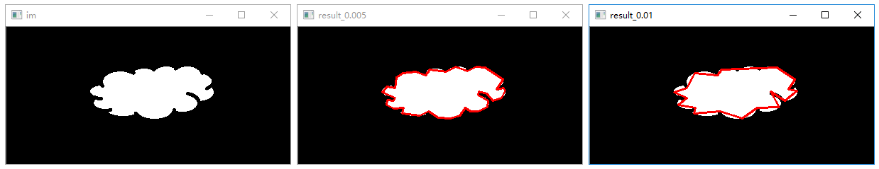
逼近多边形
函数cv2.approxPolyDP()用来构造指定精度的逼近多边形曲线。该函数的语法格式为:
1 | approxCurve = cv2.approxPolyDP(curve,epsilon,closed) |
代码:
1 | # 构建多边形,逼近轮廓 |
执行结果:
视频基本处理
读取摄像头
1 | import numpy as np |
播放视频文件
1 | import numpy as np |
捕获并保存视频
1 | import numpy as np |
综合案例
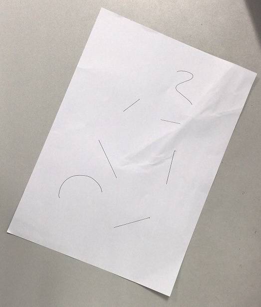
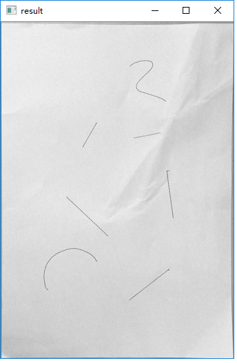
利用OpenCV实现图像校正
【任务描述】
我们对图像中的目标进行分析和检测时,目标往往具有一定的倾斜角度,自然条件下拍摄的图像,完全平正是很少的。因此,需要将倾斜的目标“扶正”的过程就就叫做图像矫正。该案例中使用的原始图像如下:
【代码】
1 | # 图像校正示例 |
【执行结果】
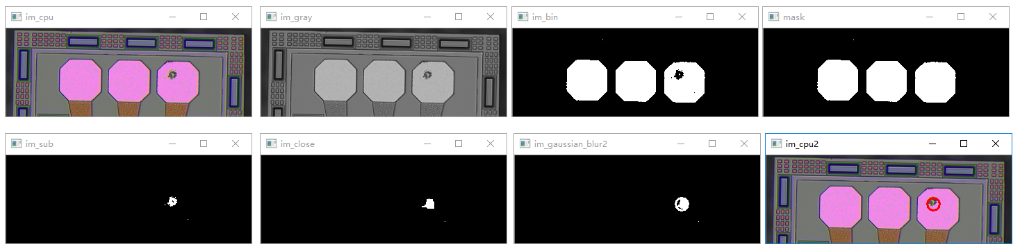
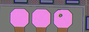
利用OpenCV检测芯片瑕疵
【任务描述】
利用图像技术,检测出芯片镀盘区域瑕疵。样本图像中,粉红色区域为镀盘区域,镀盘内部空洞为瑕疵区域,利用图像技术检测镀盘是否存在瑕疵,如果存在则将瑕疵区域标记出来。
【代码】
1 | import cv2 |
【执行结果】