决策树回归
核心思想:相似的输入必会产生相似的输出。例如预测某人薪资:
年龄:1-青年,2-中年,3-老年
年龄
学历
经历
性别
==>
薪资
1
1
1
1
==>
6000(低)
2
1
3
1
==>
10000(中)
3
3
4
1
==>
50000(高)
…
…
…
…
==>
…
1
3
2
2
==>
?
1
2
3
4
5
6
7
8
样本数量非常庞大 100 W个样本 换一种数据结构,来提高检索效率 树形结构 回归 : 均值 分类 : 投票
为了提高搜索效率,使用树形数据结构处理样本数据:
首先选择哪一个特征进行子表划分决定了决策树的性能。这么多特征,使用哪个特征先进行子表划分?
sklearn提供的决策树底层为cart树(Classification and Regression Tree),cart回归树在解决回归问题时的步骤如下:
原始数据集S,此时树的深度depth=0;
针对集合S,遍历每一个特征的每一个value(遍历数据中的所有离散值 (12个) )
用该value将原数据集S分裂成2个集合:左集合left(<=value的样本)、右集合right(>value的样本),
分别计算这2个集合的mse(均方误差),找到使(left_mse+right_mse)最小的那个value,记录下此时的特征名称和value,这个就是最佳分割特征以及最佳分割值;
mse:均方误差
((y1-y1’)^2 + (y2-y2’)^2 + (y3-y3’)^2 + (y4-y4’)^2 ) / 4 = mse
x1 y1 y1’
x2 y2 y2’
x3 y3 y3’
x4 y4 y4’
找到最佳分割特征以及最佳分割value之后,用该value将集合S分裂成2个集合,depth+=1;
针对集合left、right分别重复步骤2,3,直到达到终止条件。
决策树底层结构 为二叉树
1
2
3
4
5
终止条件有如下几种: 1 、特征已经用完了:没有可供使用的特征再进行分裂了,则树停止分裂;2 、子节点中没有样本了:此时该结点已经没有样本可供划分,该结点停止分裂;3 、树达到了人为预先设定的最大深度:depth >= max_depth,树停止分裂。4 、节点的样本数量达到了人为设定的阈值:样本数量 < min_samples_split ,则该节点停止分裂;
决策树回归器模型相关API:
1
2
3
4
5
6
7
8
9
10
import sklearn.tree as stmodel = st.DecisionTreeRegressor(max_depth=4 ) model.fit(train_x, train_y) pred_test_y = model.predict(test_x)
案例:预测波士顿地区房屋价格。
读取数据,打断原始数据集。 划分训练集和测试集。
1
2
3
4
5
6
7
8
9
10
11
12
13
14
import sklearn.datasets as sdimport sklearn.utils as suboston = sd.load_boston() print (boston.feature_names)x, y = su.shuffle(boston.data, boston.target, random_state=7 ) train_size = int (len (x) * 0.8 ) train_x, test_x, train_y, test_y = \ x[:train_size], x[train_size:], \ y[:train_size], y[train_size:]
创建决策树回归器模型,使用训练集训练模型。使用测试集测试模型。
1
2
3
4
5
6
7
8
9
10
import sklearn.tree as stimport sklearn.metrics as smmodel = st.DecisionTreeRegressor(max_depth=4 ) model.fit(train_x, train_y) pred_test_y = model.predict(test_x) print (sm.r2_score(test_y, pred_test_y))
集成算法
三个臭皮匠,顶个诸葛亮
单个模型得到的预测结果总是片面的,根据多个不同模型给出的预测结果,利用平均(回归)或者投票(分类)的方法,得出最终预测结果。
基于决策树的集成算法,就是按照某种规则,构建多棵彼此不同的决策树模型,分别给出针对未知样本的预测结果,最后通过平均或投票得到相对综合的结论。常用的集成模型包括Boosting类模型(AdaBoost、GBDT、XGBoost )与Bagging(自助聚合、随机森林)类模型。
AdaBoost模型(正向激励)
首先为样本矩阵中的样本随机分配初始权重,由此构建一棵带有权重的决策树,在由该决策树提供预测输出时,通过加权平均或者加权投票的方式产生预测值。
1
2
已经构建好一个决策树 通过1322 找到所有的女博士 一个4个 6000 8000 9000 10000 由于正向激励,对每个样本都分配了初始权重 权重为:1 1 1 3 预测: 加权均值
将训练样本代入模型,预测其输出,对那些预测值与实际值不同的样本,提高其权重,进行针对性训练,由此形成第二棵决策树。重复以上过程,构建出不同权重的若干棵决策树。
1 实际值:10000 但是你预测的为6000 构建第二个决策树,提高10000样本的权重
正向激励相关API:
1
2
3
4
5
6
7
8
9
10
11
12
13
14
15
import sklearn.tree as stimport sklearn.ensemble as semodel = st.DecisionTreeRegressor(max_depth=4 ) model = se.AdaBoostRegressor(model, n_estimators=400 , random_state=7 ) 正向激励 的基础模型 : 决策树 n_estimators:构建400 棵不同权重的决策树,训练模型 model.fit(train_x, train_y) pred_test_y = model.predict(test_x)
案例:基于正向激励训练预测波士顿地区房屋价格的模型。
1 2 3 4 5 6 7 8 model = se.AdaBoostRegressor( st.DecisionTreeRegressor(max_depth=4 ), n_estimators=400 , random_state=7 ) model.fit(train_x, train_y) pred_test_y = model.predict(test_x) print (sm.r2_score(test_y, pred_test_y))
特征重要性
作为决策树模型训练过程的副产品,根据划分子表时选择特征的顺序标志了该特征的重要程度,此即为该特征重要性指标。训练得到的模型对象提供了属性:feature_importances_来存储每个特征的重要性。
获取样本矩阵特征重要性属性:
1
2
model.fit(train_x, train_y) fi = model.feature_importances_
案例:获取普通决策树与正向激励决策树训练的两个模型的特征重要性值,按照从大到小顺序输出绘图。
1
2
3
4
5
6
7
8
9
10
11
12
13
14
15
16
17
18
19
20
21
22
23
24
25
26
27
28
29
30
31
32
33
import matplotlib.pyplot as mpmodel = st.DecisionTreeRegressor(max_depth=4 ) model.fit(train_x, train_y) fi_dt = model.feature_importances_ model = se.AdaBoostRegressor( st.DecisionTreeRegressor(max_depth=4 ), n_estimators=400 , random_state=7 ) model.fit(train_x, train_y) fi_ab = model.feature_importances_ mp.figure('Feature Importance' , facecolor='lightgray' ) mp.subplot(211 ) mp.title('Decision Tree' , fontsize=16 ) mp.ylabel('Importance' , fontsize=12 ) mp.tick_params(labelsize=10 ) mp.grid(axis='y' , linestyle=':' ) sorted_indices = fi_dt.argsort()[::-1 ] pos = np.arange(sorted_indices.size) mp.bar(pos, fi_dt[sorted_indices], facecolor='deepskyblue' , edgecolor='steelblue' ) mp.xticks(pos, feature_names[sorted_indices], rotation=30 ) mp.subplot(212 ) mp.title('AdaBoost Decision Tree' , fontsize=16 ) mp.ylabel('Importance' , fontsize=12 ) mp.tick_params(labelsize=10 ) mp.grid(axis='y' , linestyle=':' ) sorted_indices = fi_ab.argsort()[::-1 ] pos = np.arange(sorted_indices.size) mp.bar(pos, fi_ab[sorted_indices], facecolor='lightcoral' , edgecolor='indianred' ) mp.xticks(pos, feature_names[sorted_indices], rotation=30 ) mp.tight_layout() mp.show()
GBDT
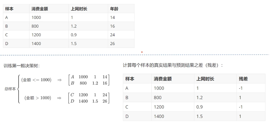
GBDT(Gradient Boosting Decision Tree 梯度提升树)通过多轮迭代,每轮迭代产生一个弱分类器,每个分类器在上一轮分类器的残差**(残差在数理统计中是指实际观察值与估计值(拟合值)之间的差)**基础上进行训练。基于预测结果的残差设计损失函数。GBDT训练的过程即是求该损失函数最小值的过程。
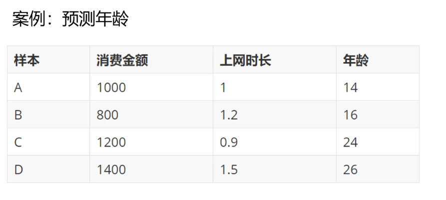
案例
原理1 :
原理2 :
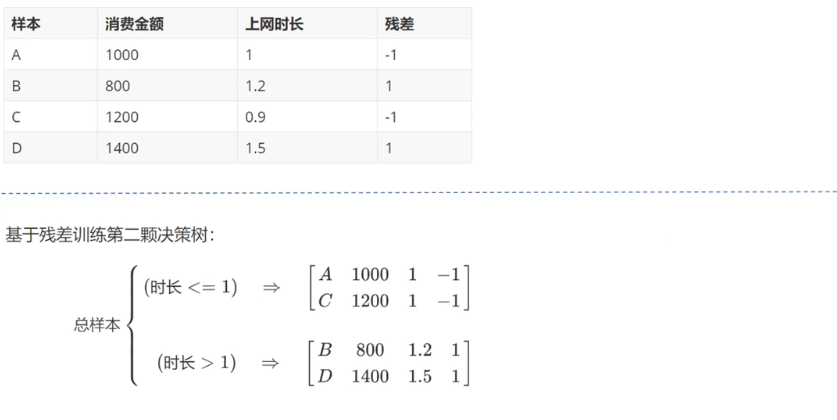
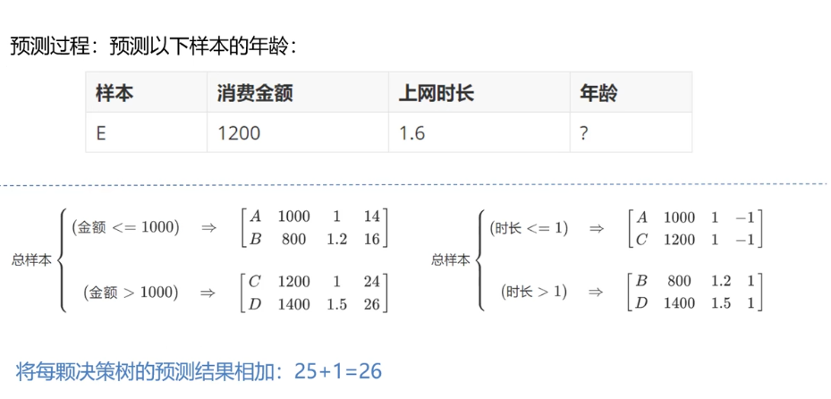
原理3 :
1
2
3
4
5
6
7
8
9
10
import sklearn.tree as stimport sklearn.ensemble as semodel = se.GridientBoostingRegressor( max_depth=10 , n_estimators=1000 , min_samples_split=2 ) model.fit(train_x, train_y) pred_test_y = model.predict(test_x)
自助聚合(BootStrap)
每次从总样本矩阵中以有放回抽样的方式随机抽取部分样本构建决策树,这样形成多棵包含不同训练样本的决策树,以削弱某些强势样本对模型预测结果的影响,提高模型的泛化特性。
因为sklearn大部分训练已经打包成了接口,很难调整每次训练的样本,所以在没有sklean接口的情况下自助聚合不容易使用。
随机森林
在自助聚合的基础上,每次构建决策树模型时,不仅随机选择部分样本,而且还随机选择部分特征,这样的集合算法,不仅规避了强势样本对预测结果的影响,而且也削弱了强势特征的影响,使模型的预测能力更加泛化。
随机森林相关API:
1
2
3
4
5
6
7
import sklearn.ensemble as semodel = se.RandomForestRegressor( max_depth=10 , n_estimators=1000 , min_samples_split=2 )
案例:分析共享单车的需求,从而判断如何进行共享单车的投放。
1
2
3
1。加载并整理数据集 2.特征分析 3.打乱数据集,划分训练集,测试集
1
2
3
4
5
6
7
8
9
10
11
12
13
14
15
16
17
18
19
20
21
22
23
24
25
26
27
28
29
30
31
32
33
34
35
36
37
38
39
40
41
42
import numpy as npimport sklearn.utils as suimport sklearn.ensemble as seimport sklearn.metrics as smimport matplotlib.pyplot as mpdata = np.loadtxt('../data/bike_day.csv' , unpack=False , dtype='U20' , delimiter=',' ) day_headers = data[0 , 2 :13 ] x = np.array(data[1 :, 2 :13 ], dtype=float ) y = np.array(data[1 :, -1 ], dtype=float ) x, y = su.shuffle(x, y, random_state=7 ) print (x.shape, y.shape)train_size = int (len (x) * 0.9 ) train_x, test_x, train_y, test_y = \ x[:train_size], x[train_size:], y[:train_size], y[train_size:] model = se.RandomForestRegressor( max_depth=10 , n_estimators=1000 , min_samples_split=2 ) model.fit(train_x, train_y) fi_dy = model.feature_importances_ pred_test_y = model.predict(test_x) print (sm.r2_score(test_y, pred_test_y))data = np.loadtxt('../data/bike_hour.csv' , unpack=False , dtype='U20' , delimiter=',' ) hour_headers = data[0 , 2 :13 ] x = np.array(data[1 :, 2 :13 ], dtype=float ) y = np.array(data[1 :, -1 ], dtype=float ) x, y = su.shuffle(x, y, random_state=7 ) train_size = int (len (x) * 0.9 ) train_x, test_x, train_y, test_y = \ x[:train_size], x[train_size:], \ y[:train_size], y[train_size:] model = se.RandomForestRegressor( max_depth=10 , n_estimators=1000 , min_samples_split=2 ) model.fit(train_x, train_y) fi_hr = model.feature_importances_ pred_test_y = model.predict(test_x) print (sm.r2_score(test_y, pred_test_y))
画图显示两组样本数据的特征重要性:
1 2 3 4 5 6 7 8 9 10 11 12 13 14 15 16 17 18 19 20 21 22 mp.figure('Bike' , facecolor='lightgray' ) mp.subplot(211 ) mp.title('Day' , fontsize=16 ) mp.ylabel('Importance' , fontsize=12 ) mp.tick_params(labelsize=10 ) mp.grid(axis='y' , linestyle=':' ) sorted_indices = fi_dy.argsort()[::-1 ] pos = np.arange(sorted_indices.size) mp.bar(pos, fi_dy[sorted_indices], facecolor='deepskyblue' , edgecolor='steelblue' ) mp.xticks(pos, day_headers[sorted_indices], rotation=30 ) mp.subplot(212 ) mp.title('Hour' , fontsize=16 ) mp.ylabel('Importance' , fontsize=12 ) mp.tick_params(labelsize=10 ) mp.grid(axis='y' , linestyle=':' ) sorted_indices = fi_hr.argsort()[::-1 ] pos = np.arange(sorted_indices.size) mp.bar(pos, fi_hr[sorted_indices], facecolor='lightcoral' , edgecolor='indianred' ) mp.xticks(pos, hour_headers[sorted_indices], rotation=30 ) mp.tight_layout() mp.show()
补充知识
R2系数详细计算
R2系数详细计算过程如下:
若用$y_i$表示真实的观测值,用$\bar{y}$表示真实观测值的平均值,用$\hat{y_i}$表示预测值则,有以下评估指标:
$$
估计值与平均值的误差,反映自变量与因变量之间的相关程度的偏差平方和.
$$
即估计值与真实值的误差,反映模型拟合程度.
$$
即平均值与真实值的误差,反映与数学期望的偏离程度.
R2_score,即决定系数,反映因变量的全部变异能通过回归关系被自变量解释的比例.计算公式:i)2}{\sum {i=1}{n} (y_i - \bar{y})^2}
R2_score = 1,样本中预测值和真实值完全相等,没有任何误差,表示回归分析中自变量对因变量的解释越好.
R2_score = 0,此时分子等于分母,样本的每项预测值都等于均值.
线性回归损失函数求导过程
线性函数定义为:w_0 - 2y w_1x_1 + w_0^2 + 2w_0w_1 x_1 + w_1^2x_1^2) \ x_1+0+2 w_0 x_1 + 2 w_1 x_1^2) \