ARO Robot Kinematics

1. Kinematic Tree, Kinematic Chain, and Forward Geometry and Backward Geometry in Robotics

1.1. Demo Case Study: Robotic Arm for Assembly Line Tasks

Super Domain: Kinematics in Robotics
Type of Method: Kinematic Analysis and Control

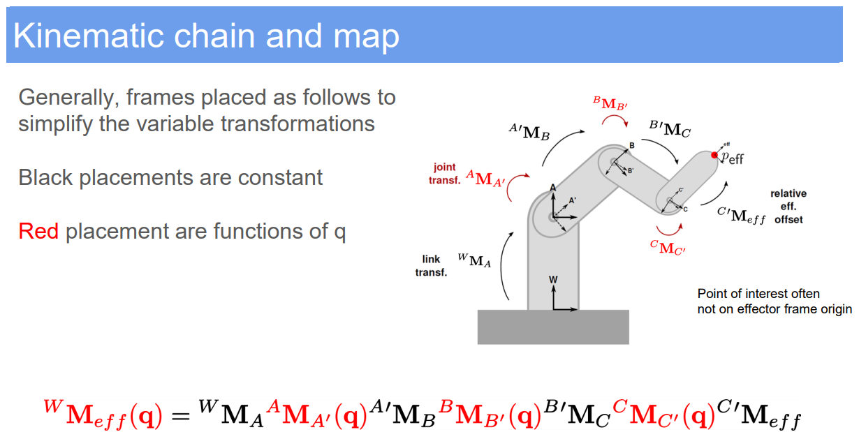
1.2. Kinematic Tree and Kinematic Chain

Objective: To model the structure and movement of a robotic arm.
Kinematic Tree:
- Represents the hierarchical structure of a robot.
- Includes all possible movements and connections between different components.
Kinematic Chain:
- A sequence of links and joints from the base to the end effector.
- Typically, a subset of the full kinematic tree, focusing on a specific task.

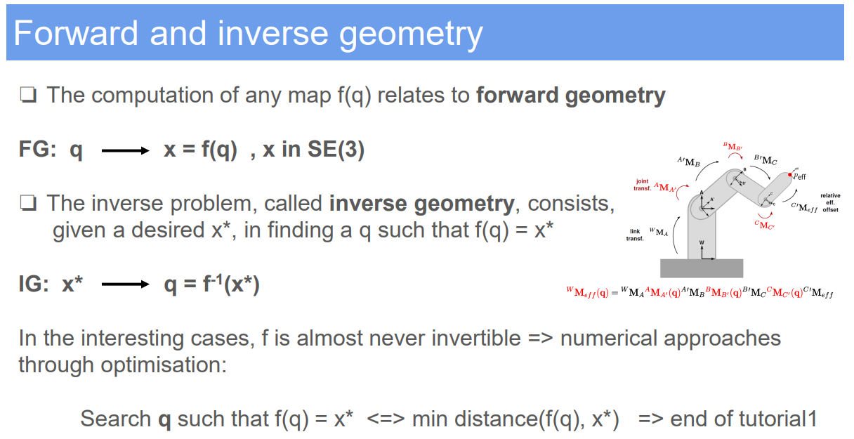
1.3. Forward Geometry

Objective: To determine the position and orientation of the robot’s end effector, given its joint parameters.
Variables:
- $\mathbf{q}$: Vector of joint parameters (angles for revolute joints, displacements for prismatic joints).
- $\mathbf{T}$: Homogeneous transformation matrix representing end effector position and orientation.
Method:
- Utilize the kinematic chain to calculate $\mathbf{T}$ as a function of $\mathbf{q}$.

1.4. Inverse Geometry

Objective: To compute the joint parameters that achieve a desired position and orientation of the end effector.
Method:
- More complex than forward kinematics, often requiring numerical methods (find inverse of forward kinematics) or iterative algorithms (check inverse kinematics).

1.5. Jacobian Matrix

Objective: To relate the velocities in the joint space to velocities in the Cartesian space.
Variables:
- $\mathbf{J}$: Jacobian matrix.
Method:
- Construct $\mathbf{J}$ such that $\dot{\mathbf{x}} = \mathbf{J} \dot{\mathbf{q}}$, where $\dot{\mathbf{x}}$ is the velocity in Cartesian space and $\dot{\mathbf{q}}$ is the velocity in joint space.

1.6. Strengths and Limitations

Strengths:
- Provides a systematic approach to model and control robotic mechanisms.
- Facilitates the understanding of complex robotic systems and their motion capabilities.
- Essential for the design and control of robotic systems in various applications.
Limitations:
- Inverse kinematics can be computationally intensive and may not have a unique solution.
- Jacobian matrices can become singular, leading to control difficulties.

1.7. Common Problems in Application

Singularities in the kinematic chain, leading to loss of control or undefined behavior.
Accuracy issues in forward and inverse kinematics due to mechanical tolerances and sensor errors.
Computational complexity, especially for robots with a high degree of freedom.

1.8. Improvement Recommendations

Implement redundancy management strategies to handle singularities.
Use advanced algorithms like pseudo-inverse or optimization-based methods for inverse kinematics.
Integrate real-time feedback and adaptive control mechanisms to compensate for inaccuracies.

s17061412162023
s17072612162023

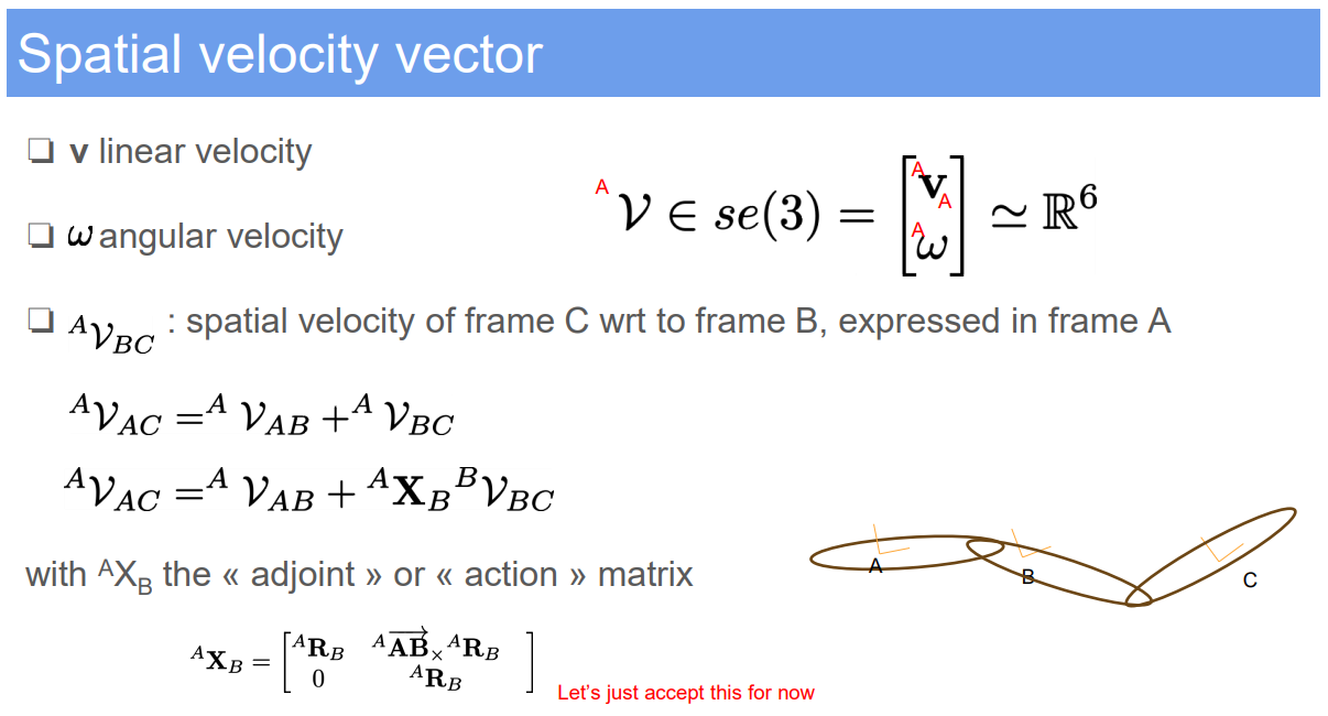
2. Spatial Velocity Vector in Robotics

2.1. Demo Case Study: Calculating the Movement of a Robotic Arm’s End Effector

Super Domain: Kinematics and Dynamics
Type of Method: Vector Analysis

2.2. Problem Definition and Variables

Objective: To represent and compute the motion of a robotic arm’s end effector through its spatial velocity, which includes both linear and angular components.
Variables:
- $\mathbf{v}$: Linear velocity component of the spatial velocity vector.
- $\mathbf{\omega}$: Angular velocity component of the spatial velocity vector.
- ${}^A\mathbf{v}_{BC}$: Spatial velocity of frame C with respect to frame B, expressed in frame A.

2.3. Assumptions

The frames of reference are rigid, with no deformation under motion.
The motion can be captured within the Euclidean space $se(3)$ framework.

2.4. Method Specification and Workflow

Spatial Velocity Representation: Use the $se(3)$ group to describe the spatial velocity as a six-dimensional vector combining linear and angular velocity.
- Representation: $\mathbf{v} \in se(3) = \begin{bmatrix} \mathbf{v}^A \ \mathbf{\omega}^A \end{bmatrix}$.
Velocity Composition: Determine the overall spatial velocity of the end effector (frame C) with respect to the base (frame A) by summing up individual velocities along the kinematic chain.
- Composition formulas:
  $$
  {}^A\mathbf{v}{AC} = {}^A\mathbf{v}{AB} + {}^A\mathbf{v}{BC}\
  {}^A\mathbf{v}{AC} = {}^A\mathbf{v}{AB} + {}^A X_B ; {}^B\mathbf{v}{BC}
  $$
Transformation Matrix Utilization: Apply the appropriate transformation matrices to express all velocities in a common frame of reference, typically the base frame.

2.5. Strengths and Limitations

Strengths:
- Provides a complete description of motion, essential for control and analysis.
- Can be used to compute velocities for any point along a robotic arm or system.
Limitations:
- Requires precise knowledge of the kinematic chain and transformations.
- The computation can become complex, especially for systems with multiple moving parts.

2.6. Common Problems in Application

Errors in calculating transformation matrices can lead to incorrect velocity composition.
The intricacy of multi-body systems can introduce challenges in real-time applications.

2.7. Improvement Recommendations

Implement software frameworks that can automatically handle spatial transformations and velocity computations.
Use state estimation techniques to accurately measure and update velocities, reducing errors from model inaccuracies.
Integrate sensor feedback for real-time correction of spatial velocities.

s17312512162023

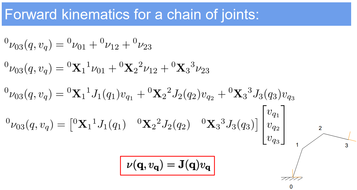
3. Forward Kinematics for a Chain of Joints

3.1. Demo Case Study: Movement Analysis of a Robotic Arm

Super Domain: Kinematics in Robotics
Type of Method: Analytical Modeling

3.2. Problem Definition and Variables

Objective: To determine the position and orientation of a robotic arm’s end effector based on joint configurations.
Variables:
- $q$: Vector of joint parameters (e.g., angles for revolute joints, displacements for prismatic joints).
- $J(q)$: Jacobian matrix at configuration $q$.
- $v(q, \dot{q})$: Velocity of the end effector in Cartesian space.
- $\dot{q}$: Vector of joint velocities.

3.3. Assumptions

The robotic arm is composed of a series of rigid bodies connected by joints, forming a kinematic chain.
The kinematic model of the robot is known and can be described by a set of parameters $q$.

3.4. Method Specification and Workflow

Jacobian Computation: Calculate the Jacobian matrix $J(q)$, which relates joint velocities to end effector velocities in Cartesian space.
Velocity Mapping: Use the Jacobian to map joint velocities $\dot{q}$ to the velocity of the end effector $v$ in Cartesian space using the formula:
- $v(q, \dot{q}) = J(q)\dot{q}$.
Local Validity: Understand that the Jacobian is only valid locally, meaning it accurately describes the relationship between joint velocities and end effector velocities only in the vicinity of the configuration $q$.

3.5. Strengths and Limitations

Strengths:
- Provides a direct and efficient way to calculate the end effector’s position and orientation.
- Essential for real-time control and path planning of robotic manipulators.
Limitations:
- The Jacobian does not provide global information about the robot’s workspace.
- Singularities in the Jacobian matrix can lead to issues in control algorithms.

3.6. Common Problems in Application

Computational complexity for robots with a high degree of freedom.
Inaccuracies in the Jacobian matrix due to modeling errors or physical changes in the robot’s structure.

3.7. Improvement Recommendations

Implement real-time Jacobian updates to accommodate changes in the robot’s configuration and avoid singularities.
Utilize redundancy in robotic design to handle singularities and increase the robustness of the kinematic model.
Integrate advanced sensors and feedback systems to refine the accuracy of the Jacobian matrix continually.

s17350612162023

4. Inverse Kinematics (IK) and Inverse Geometry (IG) in Robotics

4.1. Demo Case Study: Configuring a Robotic Arm to Reach a Target Position

Super Domain: Kinematics and Numerical Optimization
Type of Method: Mathematical Problem-Solving

4.2. Problem Definition and Variables

Objective: To determine the joint parameters that will position a robotic arm’s end effector at a desired location and orientation.
Variables:
- IK: Inverse Kinematics, focusing on finding joint velocities $\dot{q}$ to achieve a desired end-effector velocity $\nu^*$.
- IG: Inverse Geometry, solving for joint positions $q$ that reach a specific end-effector pose.
- $J(q)$: Jacobian matrix at joint configuration $q$, relating joint velocities to end-effector velocities.

4.3. Assumptions

The kinematic structure of the robotic arm is well-defined and the Jacobian matrix can be computed.

4.4. Method Specification and Workflow

IK Formulation:
- Solve $\min_{\dot{q}} | \nu(q, \dot{q}) - \nu^* |^2$, where $\nu(q, \dot{q}) = J(q)\dot{q}$.
- Utilize the Moore-Penrose pseudo-inverse $J^+$ when the Jacobian is not invertible.
IG Formulation:
- Solve $\min_q \text{dist}(^{0}M_e(q), ^{0}M_*)$ for pose and $\min_{\dot{q}} \text{dist}(^{0}M_e(q_0 \oplus \dot{q}), ^{0}M_*)$ for velocity, with $^{0}M_e$ denoting the end-effector pose in the base frame and $^{0}M_*$ being the target pose.
IK with Constraints:
- Consider velocity bounds $\dot{q}^- \leq \dot{q} \leq \dot{q}^+$ and joint limits $q^- \leq q + \Delta t \dot{q} \leq q^+$ to the optimization problem.
- Solve using a Quadratic Program (QP) solver like ‘quadprog’.

4.5. Strengths and Limitations

Strengths:
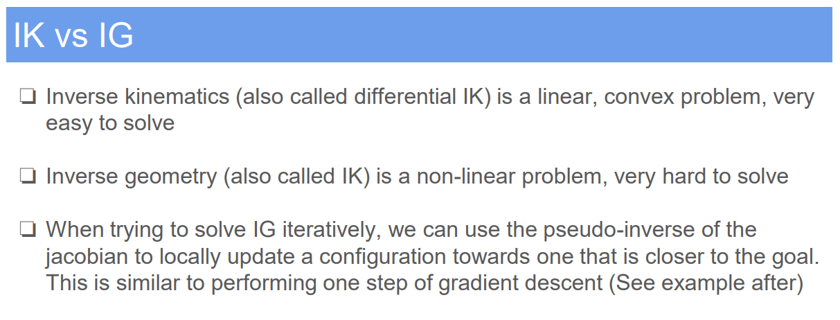
- IK is a linear problem and generally easier to solve, providing a precise control mechanism for robotic motion.
- IG offers a more direct approach to reaching a specific target pose.
Limitations:
- The Jacobian matrix may not always be invertible, necessitating pseudo-inverse solutions.
- IG is a nonlinear problem and can be computationally challenging, often requiring iterative methods.

4.6. Common Problems in Application

Jacobian singularities can lead to control problems and undefined velocities.
High computational cost for iterative solutions in IG.
Difficulty in ensuring convergence to the global minimum for IG problems.

4.7. Improvement Recommendations

Apply redundancy in the robotic design to mitigate the effects of singularities.
Use optimization libraries that are robust to numerical issues and can handle constraints effectively.
For IG, consider gradient descent methods and initialization strategies to improve convergence.

s17412512162023