1. Spring-Damper System Analysis
1.1. Demo Case Study: Vehicle Suspension System Design
- Super Domain: Mechanical Engineering and Dynamics
- Type of Method: Analytical Modeling
1.2. Problem Definition and Variables
- Objective: To design a vehicle suspension system that maximizes comfort by minimizing the impact of road irregularities on the vehicle’s passengers.
- Variables:
- $x(t)$: Displacement of the vehicle body or suspension component at time $t$.
- $m$: Mass of the vehicle or the portion of the vehicle supported by the suspension.
- $k$: Spring constant, representing the stiffness of the suspension springs.
- $c$: Damping coefficient, representing the damping properties of the shock absorbers.
- $F_{external}(t)$: External forces acting on the system, such as road bumps.
1.3. Method Specification and Workflow
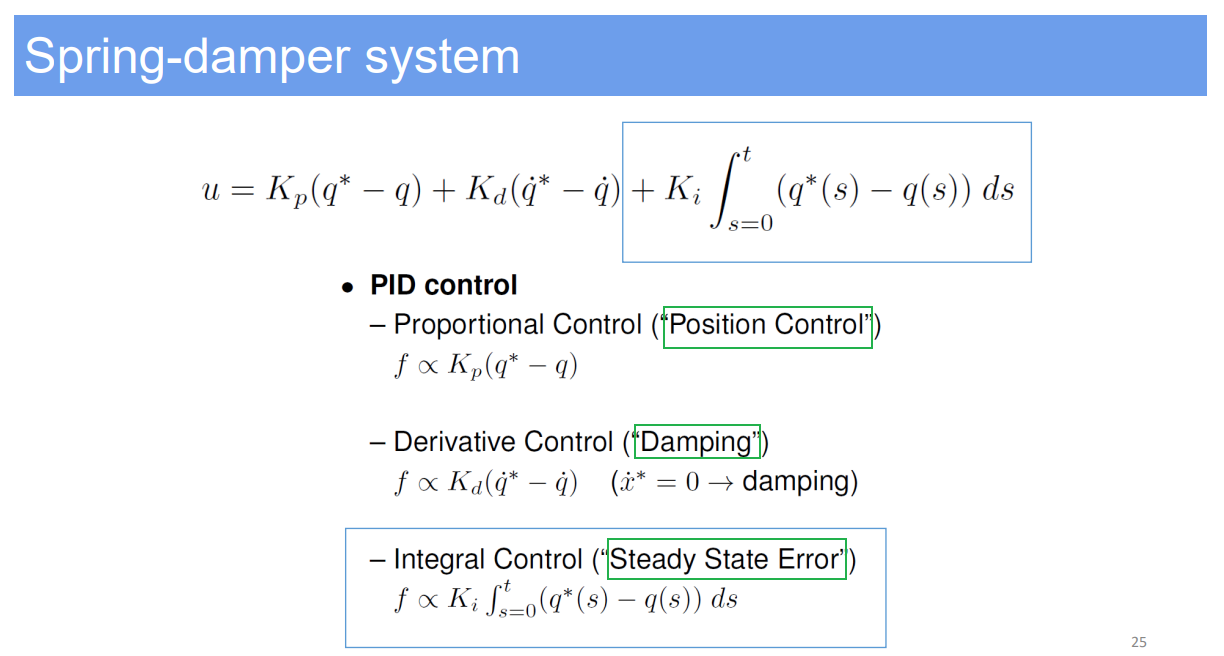
- System Dynamics: The spring-damper system’s behavior can be described by a second-order linear differential equation:
- $m\ddot{x}(t) + c\dot{x}(t) + kx(t) = F_{external}(t)$
- Analysis:
- Derive the system’s natural frequency and damping ratio to understand its free oscillation characteristics.
- Natural Frequency ($\omega_n$): $\omega_n = \sqrt{\frac{k}{m}}$
- Damping Ratio ($\zeta$): $\zeta = \frac{c}{2\sqrt{mk}}$
- Determine the system’s response to external forces, considering both transient and steady-state behavior.
- Analyze the system’s stability and performance under different loading conditions and external force profiles.
- Derive the system’s natural frequency and damping ratio to understand its free oscillation characteristics.
1.4. Strengths and Limitations
- Strengths:
- The spring-damper model is well-understood and widely applicable to various mechanical systems.
- Provides a straightforward means of designing for specific performance characteristics, like ride comfort or handling.
- Limitations:
- Simplifications in the model may not capture all real-world behaviors, such as non-linearities in the spring or damping forces.
- Assumes that all external forces are known and can be modeled, which may not be the case in unpredictable environments.
1.5. Common Problems in Application
- Non-linear behavior in the springs or damping elements can lead to deviations from the predicted response.
- Wear and environmental factors can change the system parameters over time, leading to performance degradation.
1.6. Improvement Recommendations
- Incorporate variable stiffness and damping elements to adapt to changing conditions and improve system robustness.
- Use feedback control systems, like semi-active or active suspensions, to dynamically adjust the system’s response.
1.7. Discussion on Spring-Damper Systems
Spring-damper systems form the basis of many mechanical systems designed to absorb energy and mitigate the transmission of shock and vibration. In the context of vehicle suspensions, the interplay between the spring and damper is critical for ensuring that the vehicle can maintain contact with the road surface while providing a smooth ride.
Optimizing a spring-damper system involves a trade-off between stiffness for handling and softness for comfort. The correct balance depends on the intended use of the vehicle; for example, a sports car may have a stiffer setup for better handling, while a luxury car may prioritize a softer setup for comfort.
Advanced systems may include additional components like anti-roll bars for improved stability or pneumatic or hydraulic systems for adjustable ride height and stiffness. The design process is iterative and often relies on both computational models and real-world testing to fine-tune the system for the desired performance outcomes.

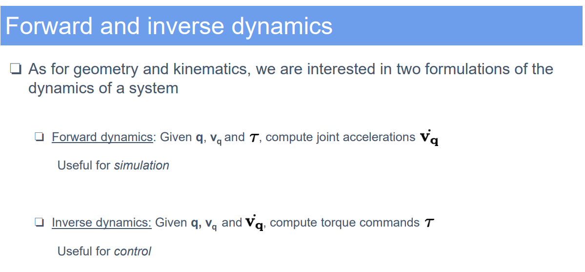
2. Robotics Dynamics
2.1. Demo Case Study: Industrial Robotic Arm for Assembly Line
- Super Domain: Robotics and Mechanical Systems
- Type of Method: Physics-based Modeling
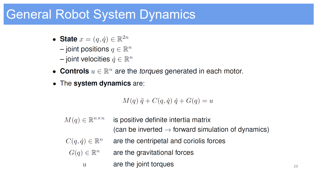
2.2. Problem Definition and Variables
- Objective: To accurately predict and control the motion of an industrial robotic arm used in an assembly line, taking into account the forces and torques acting on it.
- Variables:
- $q$: Vector of joint positions.
- $\dot{q}$: Vector of joint velocities.
- $\ddot{q}$: Vector of joint accelerations.
- $\tau$: Vector of torques applied at the joints.
- $M(q)$: Inertia matrix.
- $C(q, \dot{q})$: Coriolis and centrifugal forces matrix.
- $G(q)$: Gravity vector.
2.3. Method Specification and Workflow
- Dynamics Equations: Use the Euler-Lagrange or Newton-Euler formulations to derive the equations of motion for the robotic arm.
- Euler-Lagrange Formulation:
$\frac{d}{dt} \left( \frac{\partial L}{\partial \dot{q}} \right) - \frac{\partial L}{\partial q} = \tau$
where $L$ is the Lagrangian representing the difference between kinetic and potential energies. - Newton-Euler Formulation:
$M(q)\ddot{q} + C(q, \dot{q})\dot{q} + G(q) = \tau$
- Euler-Lagrange Formulation:
- Simulation: Integrate the equations of motion to simulate the arm’s behavior under various control strategies.
- Control: Design control laws (like PID controllers, feedforward control, computed torque control) to achieve desired motion trajectories.
2.4. Strengths and Limitations
- Strengths:
- Provides a detailed and accurate model of the robot’s physical behavior.
- Enables the design of efficient and responsive control systems.
- Limitations:
- Complex and highly nonlinear equations can be challenging to solve in real-time.
- Requires precise knowledge of all system parameters, which may not always be available or may change over time.
2.5. Common Problems in Application
- Uncertainties in model parameters like inertia and friction can lead to control inaccuracies.
- External disturbances and unmodeled dynamics can degrade performance.
2.6. Improvement Recommendations
- Use model identification techniques to refine the parameters in the dynamic model.
- Implement robust or adaptive control strategies to handle model uncertainties and external disturbances.
2.7. Discussion on Robotics Dynamics
The dynamics of robotics is a critical aspect that intersects with various disciplines, such as mechanical engineering, control theory, and computer science. It involves the application of classical mechanics to predict the behavior of robots, which is essential for designing control systems that can accurately guide their movements.
The dynamic model’s complexity can vary significantly based on the robot’s structure. For instance, a simple two-link planar arm has a much simpler model than a humanoid robot. Advanced robots require sophisticated models that account for the interplay between dynamics and control systems, especially when interacting with complex or uncertain environments.
In practical applications, the dynamics of robotics is often coupled with real-time sensing and feedback mechanisms to allow the robot to interact with its surroundings adaptively. This integration is pivotal in modern robotics applications, such as autonomous vehicles, drones, and interactive robotic systems.
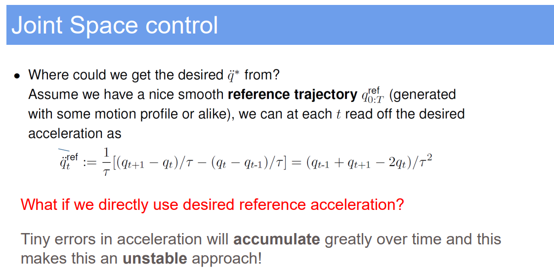
3. Joint Space Control Method
3.1. Demo Case Study: Articulated Robotic Arm for Precision Assembly
- Super Domain: Robotics and Control Engineering
- Type of Method: Control Strategy
3.2. Problem Definition and Variables
- Objective: Control an articulated robotic arm to follow a desired trajectory with high precision for tasks requiring fine manipulation, such as in precision assembly lines.
- Variables:
- $q$: Vector of joint angles or displacements.
- $\dot{q}$: Vector of joint velocities.
- $\ddot{q}$: Vector of joint accelerations.
- $\tau$: Vector of torques or forces applied to the robot’s joints.
- $q_{desired}$: Desired trajectory for each joint, defined as a function of time. We can get this with PID control or as spring damper system.
3.3. Method Specification and Workflow
- Control Strategy: Employ a feedback control loop to ensure that each joint of the robotic arm follows the desired trajectory as closely as possible.
- Workflow:
- Define the desired trajectory for each joint in terms of position, velocity, and acceleration.
- Measure the current state of each joint.
- Calculate the error between the desired and actual joint states.
- Apply a control law (such as PID control) to compute the control input $\tau$ for each joint to correct the error.
- Adjust the control inputs based on dynamic models of the robotic arm to account for the interactions between joints due to the arm’s mechanics.
- Update the control inputs at each time step to continuously correct the trajectory.
3.4. Strengths and Limitations
- Strengths:
- Direct control of each joint allows for straightforward implementation and interpretation.
- Effective for systems where precise control over individual joint movements is necessary.
- Well-suited for tasks with well-defined joint trajectories.
- Limitations:
- May not consider the overall posture of the robot or the end-effector’s position in Cartesian space.
- Less efficient for tasks that require complex interaction with the environment or end-effector orientation control.
3.5. Common Problems in Application
- Coupling between joints can lead to complex dynamics that are challenging to control precisely.
- Variations in load or external disturbances can affect joint performance and lead to deviations from the desired trajectory.
3.6. Improvement Recommendations
- Implement feedforward control strategies alongside feedback control to anticipate and compensate for known system dynamics.
- Use real-time adaptive control to adjust for model uncertainties and external disturbances dynamically.
3.7. Joint Space Control Discussion
Joint space control is particularly advantageous when the precise motion of each joint is the primary objective, rather than the specific path the end-effector takes through Cartesian space. This approach is common in industrial robotics, where the robot’s tasks are often broken down into a sequence of joint movements, and the end-effector’s path is less critical than its final position or orientation.
In practice, joint space control requires accurate models of the robotic arm’s dynamics, including the mass and inertia of the limbs, friction in the joints, and any flex in the structure. These models are used to predict how the robot will move in response to the applied torques and to design control laws that can achieve the desired movements.
Despite its widespread use, joint space control does have limitations, particularly when dealing with complex tasks that require the robot to interact with its environment in more sophisticated ways. For such tasks, Cartesian space control methods, which focus on the position and orientation of the end-effector in 3D space, may be more appropriate. However, for many applications, especially those with repetitive and well-defined movements, joint space control remains a robust and effective strategy.
4. Lagrangian Dynamics
4.1. Demo Case Study: Modeling a Bipedal Humanoid Robot
- Super Domain: Theoretical Mechanics and Robotics
- Type of Method: Analytical Dynamics Modeling
4.2. Problem Definition and Variables
- Objective: Develop a dynamic model for a bipedal humanoid robot to understand the forces and motions involved in tasks such as walking, running, or climbing.
- Variables:
- $q$: Generalized coordinates representing the robot’s configuration.
- $\dot{q}$: Generalized velocities, the time derivatives of the coordinates.
- $L$: Lagrangian, defined as the difference between the kinetic energy $T$ and potential energy $V$ of the system, $L = T - V$.
- $\tau$: Generalized forces acting on the system.
4.3. Method Specification and Workflow
- Lagrangian Formulation: Use the Lagrangian function to derive the equations of motion.
- $\frac{d}{dt}\left(\frac{\partial L}{\partial \dot{q}_i}\right) - \frac{\partial L}{\partial q_i} = \tau_i$, for $i = 1$ to $n$, where $n$ is the number of degrees of freedom.
- Workflow:
- Identify and label all degrees of freedom for the robot.
- Define the kinetic and potential energy expressions in terms of the generalized coordinates and velocities.
- Compute the partial derivatives of the Lagrangian with respect to each coordinate and velocity.
- Apply the Lagrange equations to derive the second-order differential equations of motion.
- Solve the equations of motion for the generalized coordinates as functions of time to predict the robot’s motion under various conditions.
4.4. Strengths and Limitations
- Strengths:
- Provides a systematic approach to deriving equations of motion for complex, multi-body systems.
- Avoids the need to directly deal with the internal forces and moments between components of the system.
- Limitations:
- Can be algebraically complex, especially for systems with many degrees of freedom.
- Requires accurate knowledge of all system parameters, such as masses, moments of inertia, and geometry.
4.5. Common Problems in Application
- Computational difficulty in solving the resulting differential equations, particularly for non-linear systems.
- Sensitivity to parameter variations, which can lead to significant errors in the predicted motions.
4.6. Improvement Recommendations
- Use computational tools like symbolic mathematics software for deriving and solving the Lagrange equations.
- Combine with experimental data for system identification to refine the model and improve accuracy.
4.7. Lagrangian Dynamics: Discussion
Lagrangian dynamics is an elegant and powerful framework that is particularly useful in robotics for analyzing systems where direct measurement of forces is challenging. By focusing on energy rather than forces, the Lagrangian approach simplifies the modeling process and is especially beneficial for understanding the motion of articulated robots like bipedal humanoids.
This approach allows for the decoupling of the robot’s motion into individual components, which can be particularly advantageous when considering complex interactions within the robot’s structure or between the robot and its environment. Additionally, it provides a foundation for developing advanced control strategies, such as those needed for balance and gait control in bipedal locomotion.
However, the complexity of the Lagrangian formulation increases significantly with the complexity of the robot’s structure. For systems with a large number of interconnected parts, the equations can become unwieldy, and numerical methods may be required to solve them. Despite this, the insights gained from a Lagrangian-based analysis are invaluable for the design, optimization, and control of robotic systems.
5. Newton-Euler Dynamics
5.1. Demo Case Study: Real-Time Dynamics for Mobile Robotics
- Super Domain: Mechanics and Robotics
- Type of Method: Analytical Dynamics Modeling
5.2. Problem Definition and Variables
- Objective: Formulate the dynamics of a mobile robot for real-time applications, such as navigation and manipulation, by considering the forces and moments acting on the robot.
- Variables:
- $F$: Vector of external forces applied to the robot.
- $\tau$: Vector of external torques applied to the robot.
- $m$: Mass of the robot or robot component.
- $I$: Inertia tensor of the robot or component.
- $a$: Linear acceleration of the robot’s center of mass.
- $\alpha$: Angular acceleration of the robot.
- $v$: Linear velocity of the robot’s center of mass.
- $\omega$: Angular velocity of the robot.
5.3. Method Specification and Workflow
- Newton-Euler Equations: Use Newton’s second law for translation and Euler’s equations for rotation to model the robot’s dynamics.
- Translation: $F = m a$
- Rotation: $\tau = I \alpha + \omega \times (I \omega)$
- Workflow:
- Identify all forces and torques acting on the robot, including gravity, friction, and interaction with the environment.
- Decompose the motion into translational and rotational components.
- Apply Newton’s second law to each body or component of the robot to find linear acceleration.
- Apply Euler’s equations to find angular acceleration.
- Integrate acceleration to find velocity and position for motion planning and control purposes.
5.4. Strengths and Limitations
- Strengths:
- Directly applicable to rigid body dynamics and intuitive to understand.
- Suitable for systems where forces and torques are readily measurable or estimable.
- Facilitates the decoupling of translational and rotational dynamics, which simplifies analysis and control.
- Limitations:
- Requires the assumption of rigid bodies, which may not be valid for robots with flexible parts.
- Can become computationally expensive for systems with many interconnected bodies.
5.5. Common Problems in Application
- Difficulties arise in modeling systems with significant elasticity or deformability.
- Measurement errors in force and torque can lead to inaccuracies in the predicted dynamics.
5.6. Improvement Recommendations
- Implement recursive Newton-Euler algorithms for computational efficiency in systems with multiple interconnected bodies.
- Use sensor fusion techniques to improve the accuracy of force and torque measurements.
5.7. Newton-Euler Dynamics: Discussion
The Newton-Euler method is one of the fundamental approaches to modeling the dynamics of robotic systems. It’s particularly useful in scenarios where the robot interacts with its environment dynamically, such as in manipulation tasks or when traversing uneven terrain.
For mobile robotics, where the dynamics can drastically affect navigation and stability, Newton-Euler dynamics provide a framework to ensure that all forces, including those resulting from collisions or interactions with various surfaces, are accounted for in the robot’s control system.
In practice, while the Newton-Euler equations provide a rich description of motion, they often need to be supplemented with additional constraints or models to account for non-rigid behaviors, complex geometries, and real-world uncertainties. Advances in computational power and algorithms continue to expand the practical applicability of Newton-Euler dynamics in robotics.
6. Canonical Form for Articulated Rigid Bodies
6.1. Demo Case Study: Dynamics of a Multi-Joint Robotic Arm
- Super Domain: Robotics Dynamics
- Type of Method: Analytical Dynamics
6.2. Problem Definition and Variables
- Objective: To describe the motion of a multi-joint robotic arm, taking into account the interactions between its articulated rigid bodies.
- Variables:
- $q$: Vector of joint displacements.
- $\dot{q}$: Vector of joint velocities.
- $\ddot{q}$: Vector of joint accelerations.
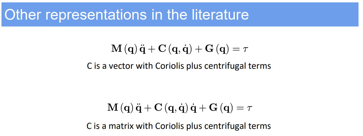
- $M(q)$: Inertia matrix, depending on the configuration $q$.
- $B(q)[\dot{q}]$: Coriolis matrix, a function of configuration $q$ and velocities $\dot{q}$.
- $C(q)[\dot{q}^2]$: Centrifugal matrix, a function of configuration $q$ and the square of velocities $\dot{q}$.
- $G(q)$: Gravity vector, dependent on the configuration $q$.
- $\tau$: Vector of external forces and torques applied to the joints.
6.3. Method Specification and Workflow
- Canonical Form Equations: The equations that describe the dynamics of articulated rigid bodies in their canonical form are:
- $M(q) \ddot{q} + B(q)[\dot{q}] + C(q)[\dot{q}^2] + G(q) = \tau$
- Workflow:
- Determine the system’s configuration and calculate the inertia matrix $M(q)$.
- Compute the Coriolis and centrifugal forces using matrices $B(q)$ and $C(q)$, respectively.
- Evaluate the gravity vector $G(q)$ based on the current configuration.
- Use these terms to solve for the joint accelerations $\ddot{q}$ given the external forces/torques $\tau$.
- Integrate the joint accelerations over time to obtain velocities and displacements for trajectory planning and control.
6.4. Strengths and Limitations
- Strengths:
- Provides a complete and systematic approach to modeling the dynamics of complex articulated systems.
- The canonical form separates different dynamic effects, which is useful for control and simulation purposes.
- Limitations:
- The complexity of the matrices involved can lead to computationally intensive calculations, especially for systems with many degrees of freedom.
- Requires accurate parameters for the inertia matrix and knowledge of external forces, which may not always be available.
6.5. Common Problems in Application
- Computational challenges in real-time applications due to the complexity of the matrices.
- Difficulties in measuring and estimating the parameters accurately in a real-world environment.
6.6. Improvement Recommendations
- Optimize the computational algorithms for real-time application, possibly using parallel computing techniques or simplifying assumptions.
- Combine with sensor data for parameter estimation and to account for unmodeled dynamics in control strategies.
6.7. Canonical Form for Articulated Rigid Bodies: Discussion
The canonical form for articulated rigid bodies is essential in robotics for understanding how the parts of a robotic system influence each other’s motion. This formulation is particularly critical when designing controllers for robots that need to perform precise and complex tasks, as it directly relates the control inputs (forces/torques) to the resulting motion of the robot.
In practical scenarios, such as in the manufacturing industry, the canonical form helps in simulating the robot’s behavior before actual deployment, which ensures safety and efficiency. It also provides a foundation for advanced control techniques, like model predictive control (MPC) or computed torque control, which can greatly enhance the performance of robotic systems.
The canonical form also serves as a bridge between the physical robot and digital simulation tools, enabling the development and testing of robotic systems within virtual environments. This greatly speeds up the design process and allows for the optimization of robot performance without the need for extensive physical prototypes.
7. Is Canonical Form for Articulated Rigid Bodies based on Newton-Euler dynamics?
Yes, the Canonical Form for Articulated Rigid Bodies is indeed based on Newton-Euler dynamics. The Newton-Euler approach provides the foundational principles for the forces and torques acting on each rigid body within a mechanical system. The Canonical Form for Articulated Rigid Bodies takes these principles and organizes them into a more structured and matrix-based representation that is particularly suited for complex, interconnected systems like robotic arms.
In essence, the Canonical Form encapsulates the Newtonian mechanics (Newton’s laws for translational motion and Euler’s laws for rotational motion) within a framework that is more convenient for computational modeling and control of articulated systems. It transforms the individual body dynamics described by Newton-Euler into a system-level description that accounts for the interactions between bodies due to their articulation.
To summarize:
- Newton-Euler dynamics provides the individual equations of force and torque balance for each rigid body.
- The Canonical Form aggregates these into a holistic model using matrices, making it suitable for systems with multiple interacting bodies, such as robots with several joints and links.
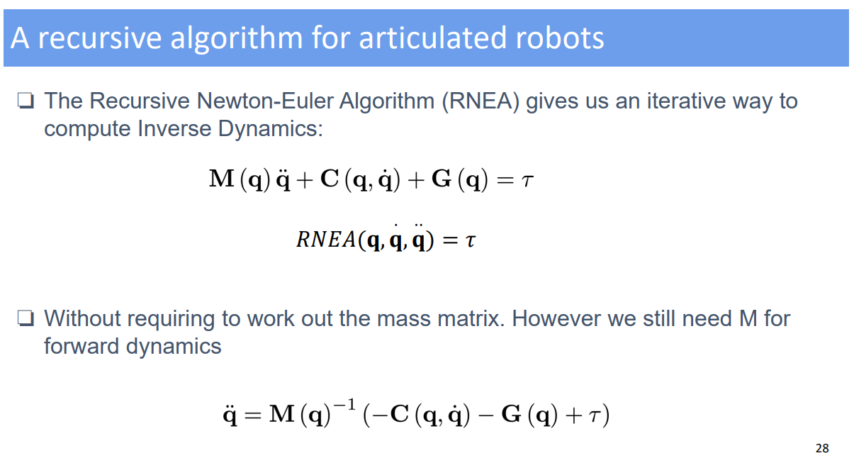
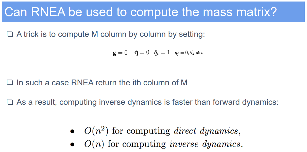
8. Recursive Newton-Euler Algorithm (RNEA) using Canonical Form
8.1. Demo Case Study: Dynamic Response of a Multi-Joint Robotic Manipulator
- Super Domain: Robotics Dynamics
- Type of Method: Computational Dynamics for Inverse Dynamics
8.2. Problem Definition and Variables
- Objective: To calculate the inverse dynamics of a multi-joint robotic manipulator efficiently, providing the joint torques needed for a given movement.
- Variables:
- $q$: Vector of joint positions.
- $\dot{q}$: Vector of joint velocities.
- $\ddot{q}$: Vector of joint accelerations.
- $M(q)$: Inertia matrix as a function of the joint configuration $q$.
- $C(q)$: Coriolis and centrifugal forces matrix, dependent on the configuration $q$ and joint velocities $\dot{q}$.
- $G(q)$: Gravity vector, a function of the joint configuration $q$.
- $\tau$: Vector of joint torques resulting from external forces and moments.
8.3. Method Specification and Workflow
- Algorithmic Approach: The RNEA uses the kinematic chain of the robot to calculate joint torques through two recursive passes, one to compute velocities and accelerations and another for forces and torques.
- Workflow:
- Initialization: Set base velocities and accelerations to zero: $\dot{q}_0 = 0$, $\ddot{q}_0 = 0$.
- Forward Recursion: Compute velocities and accelerations for each joint/link.
- $\dot{v}i = \dot{v}{i-1} + \ddot{q}i \times r{i-1} + \dot{q}_i \times (\dot{q}i \times r{i-1})$
- $\dot{\omega}i = \dot{\omega}{i-1} + \ddot{q}_i$
- Backward Recursion: Compute joint forces and torques from the end-effector to the base.
- $f_i = M_i \dot{v}_i + C_i(\dot{q}_i) \times \dot{q}_i + G_i$
- $\tau_i = f_{i-1} \times r_{i-1} + f_i \times r_i + \tau_{ext,i}$
- Output: The resulting $\tau$ vector represents the joint torques needed to produce the desired motion.
8.4. Strengths and Limitations
- Strengths:
- Algorithmic efficiency makes it suitable for real-time applications.
- Can handle complex, multi-joint robotic systems.
- Limitations:
- Relies on accurate modeling of the robot’s physical parameters.
- Assumes rigid bodies, which may not account for all dynamics in flexible or soft robotic systems.
8.5. Common Problems in Application
- Errors in parameter estimation can lead to inaccurate torque computations.
- Real-world factors such as joint friction or unmodeled dynamics can affect the results.
8.6. Improvement Recommendations
- Enhance parameter estimation through sensor data integration.
- Implement control strategies that can compensate for real-world discrepancies from the modeled dynamics.
9. Why the torque in backward recursion of RNEA add i-1 term?
In the backward recursion step of the Recursive Newton-Euler Algorithm (RNEA), the torque for each joint is calculated by considering both the force applied to the current joint/link and the forces from the subsequent joints/links. The reason for including the $f_{i-1}$ term (forces from the previous joint) when calculating $\tau_i$ is to account for the dynamic effects that propagate along the kinematic chain of the robot.
When calculating the torque at joint $i$, you must consider not only the direct forces and moments acting on that joint but also the effects of all the forces and moments acting on all the links that follow joint $i$ in the kinematic chain. This is because the motion of each link affects the motion of all subsequent links. Therefore, the torques at each joint are the result of both the local forces/moments and the transmitted forces/moments from all subsequent joints and links.
The term $f_{i-1} \times r_{i-1}$ represents the moment due to the force at the previous joint/link acting at a distance $r_{i-1}$ from the current joint. This term ensures that the torques calculated include these transmitted forces, which are crucial for accurately determining the net torque required at each joint to achieve the desired motion.
This recursive accumulation of forces and moments from the end-effector back to the base is what allows RNEA to be so efficient and accurate for calculating the inverse dynamics of articulated robotic systems.
Reference: The University of Edinburgh, Advanced Robotics, course link
Author: YangSier (discover304.top)
🍀碎碎念🍀
Hello米娜桑,这里是英国留学中的杨丝儿。我的博客的关键词集中在编程、算法、机器人、人工智能、数学等等,持续高质量输出中。
🌸唠嗑QQ群:兔叽の魔术工房 (942848525)
⭐B站账号:白拾Official(活跃于知识区和动画区)
Cover image credit to AI generator.