ARO Robot Controller

1. First-Order Error Dynamics (PD control)

1.1. Demo Case Study: Velocity Control of a Mass-Damper System

Super Domain: Control Systems, Dynamics
Type of Method: Error Dynamics Analysis

1.2. Problem Definition with Variables Notations

Objective: Analyze the error dynamics of a system to predict how the system responds to a change from a desired state, focusing on velocity control.
Variables:
- $\theta_e$: Error in position or angle.
- $\dot{\theta}_e$: Error in velocity.
- $m$: Mass of the object.
- $b$: Damping coefficient.
- $k$: Spring constant.
- $t$: Time constant, where $t = \frac{b}{k}$.

1.3. Assumptions

The system behaves according to linear dynamics.
No external forces are acting on the system except for the spring and damper.

1.4. Method Specification and Workflow

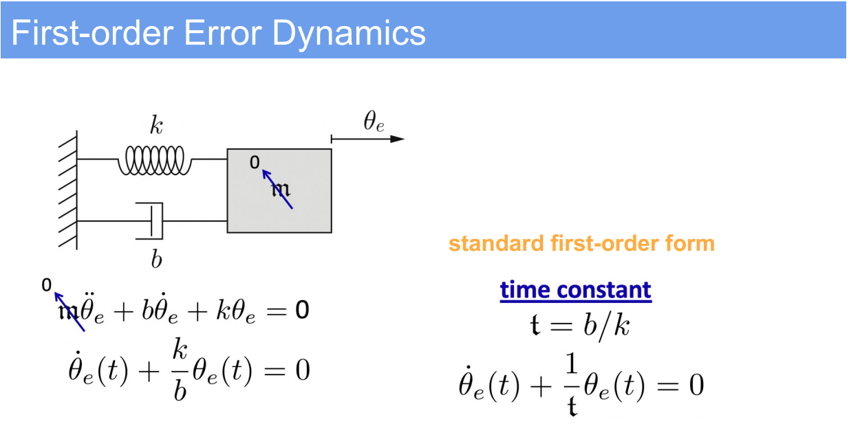
Standard Form of First-Order ODE:
- The error dynamics are described by a first-order ordinary differential equation (ODE):
  $\dot{\theta}_e(t) + \frac{k}{b} \theta_e(t) = 0$
Time Constant:
- The time constant $t$ is a measure of how quickly the system responds to changes in the error. It’s defined as the time it takes for the error to decrease by a factor of $e$ (Euler’s number) from its initial value.

1.5. Comment: Strengths and Limitations

Strengths:
- First-order error dynamics are relatively simple to analyze and provide insights into system behavior.
- The time constant gives a straightforward measure of the system’s responsiveness.
Limitations:
- Assumes a linear relationship, which may not hold for all real-world systems, especially those with nonlinear characteristics or significant external disturbances.

1.6. Common Problems When Applying the Method

Oversimplification of complex dynamics can lead to inaccurate predictions.
Damping ratio and natural frequency are not considered, which are important in second-order systems.

1.7. Improvement Recommendations

For systems where higher-order dynamics are significant, use higher-order differential equations for analysis.
Incorporate adaptive control techniques to handle systems with varying parameters or non-linear behavior.

1.8. Discussion on First-Order Error Dynamics

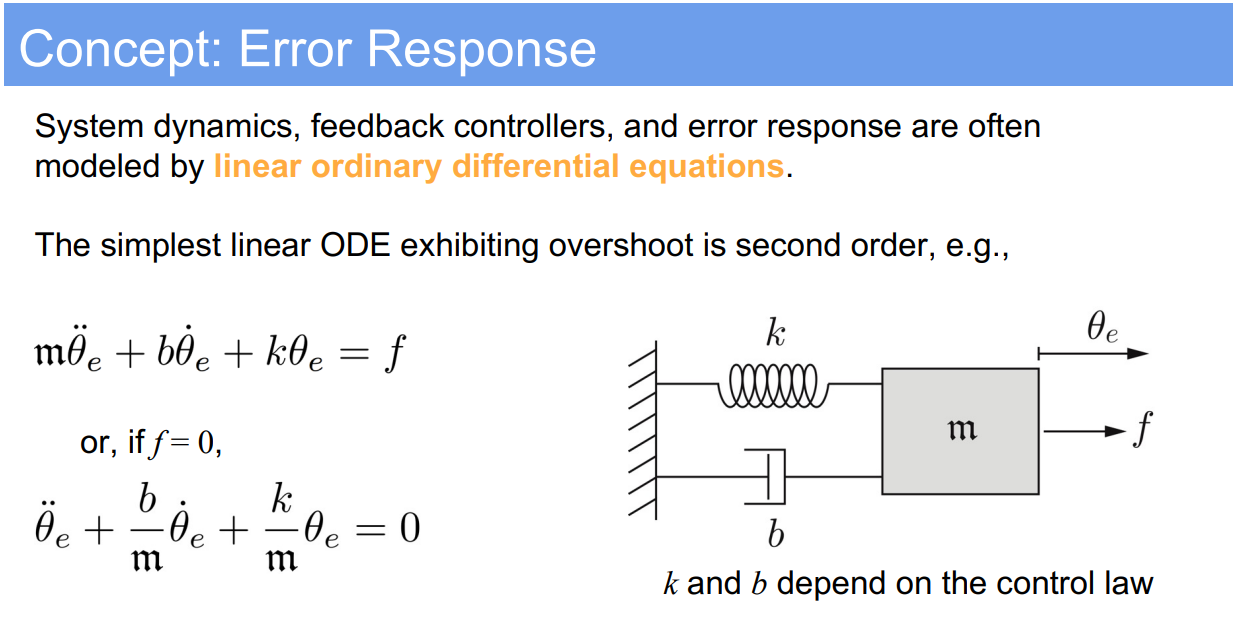
The first-order error dynamics provide a basic understanding of how a system will respond to errors in velocity. The damping coefficient $b$ plays a crucial role in determining the rate at which the error will decay. A larger $b$ results in a faster error decay, which can be desirable for quickly stabilizing a system but may lead to higher energy consumption or more aggressive control actions.

In practical applications, the first-order error dynamics can be used to design feedback controllers that effectively reduce velocity errors, such as in automated manufacturing systems where precise speed control is necessary. It’s also useful in robotics for controlling the velocity of actuators or motors.

The concept of time constant $t$ is particularly useful for tuning controllers in a first-order system, providing a direct relationship between the system parameters and the desired speed of response. However, for more complex systems, this first-order model may need to be expanded or used in conjunction with other control strategies to achieve the desired control performance.

s20523312162023

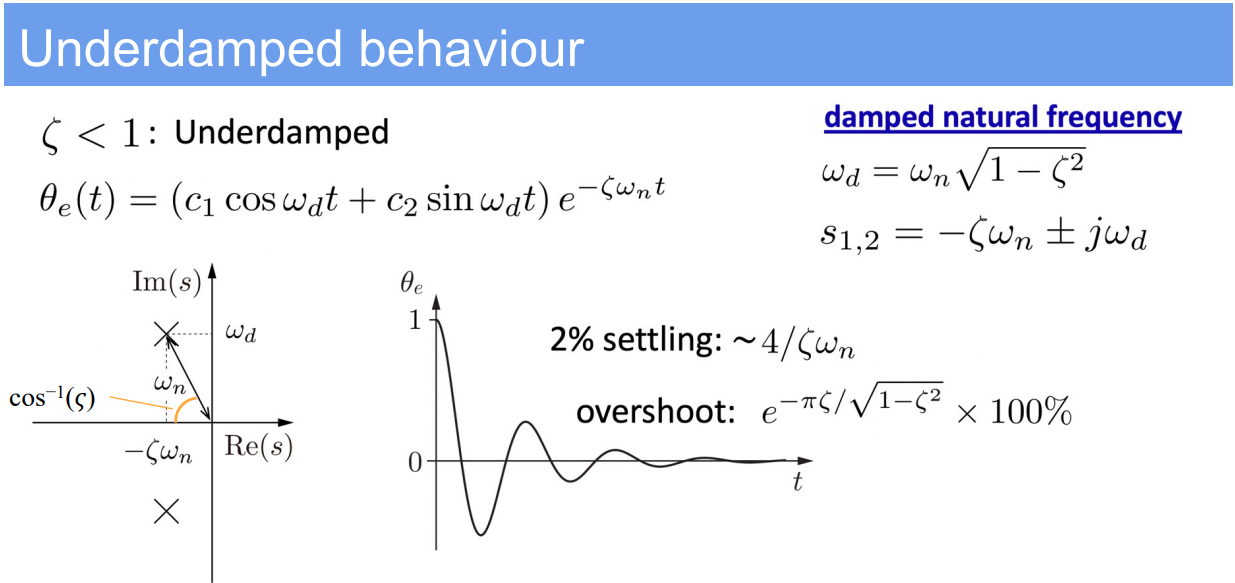
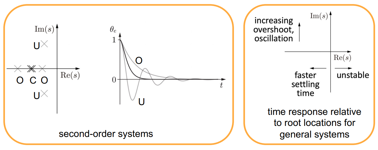
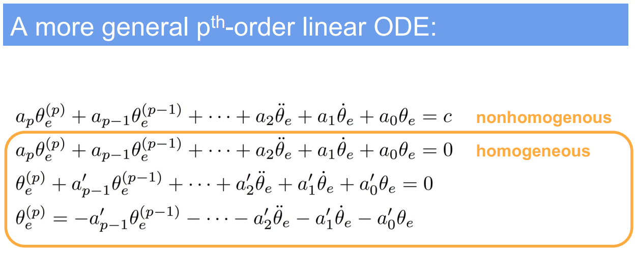
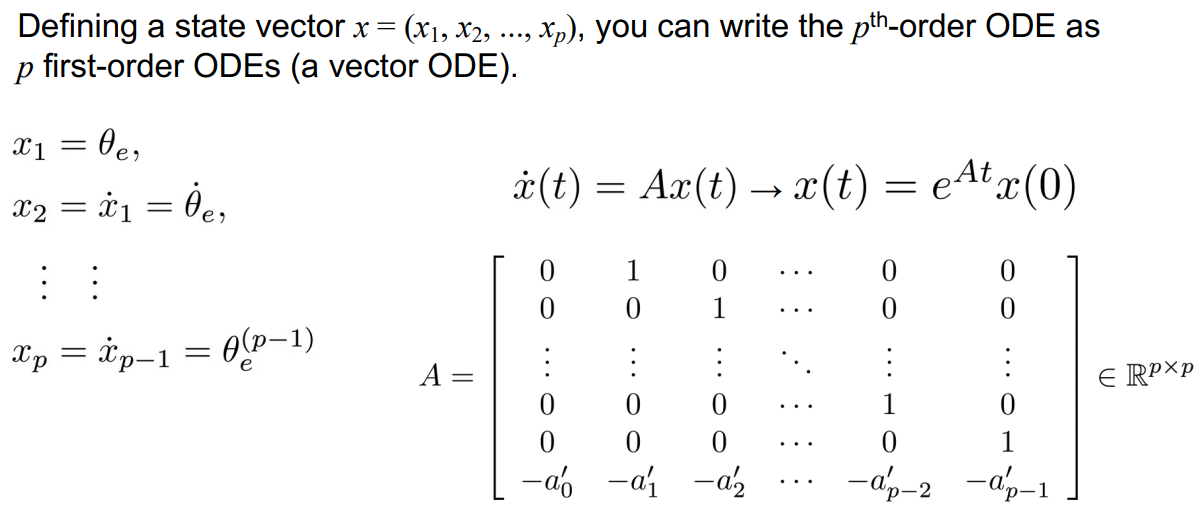
2. Second-Order Error Dynamics (PID control)

Case Study: Modeling the response of a system with acceleration considered, typically seen in mechanical systems with mass, damping, and spring constants.

Super Domain: Control Systems, specifically in the context of mechanical systems with mass-spring-damper assemblies.
Method Level/Type: Second-order linear ordinary differential equation representing physical systems.

2.1. Problem Definition:

Variables:
- $\theta_e(t)$: Error in position at time $t$.
- $\dot{\theta}_e(t)$: Error in velocity at time $t$.
- $\ddot{\theta}_e(t)$: Error in acceleration at time $t$.
- $k$: Spring constant.
- $b$: Damping coefficient.
- $m$: Mass of the object.
- $\omega_n$: Natural frequency of the system.
- $\zeta$: Damping ratio of the system.

2.2. Assumptions:

The system is modeled as a linear second-order system.
No external forces acting on the system (homogeneous equation).
The system parameters $m$, $b$, and $k$ are constant over time.

2.3. Method Specification and Workflow:

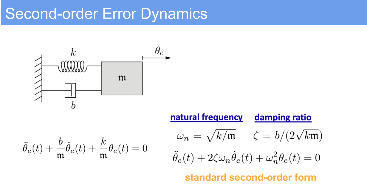
Standard form of the second-order differential equation:
$$
m\ddot{\theta}_e + b\dot{\theta}_e + k\theta_e = 0
$$
This can be rewritten using the standard form variables as:
$$
\ddot{\theta}_e + 2\zeta\omega_n\dot{\theta}_e + \omega_n^2\theta_e = 0
$$
The solution involves calculating the system’s natural frequency $\omega_n$ and damping ratio $\zeta$, which are given by:
$$
\omega_n = \sqrt{\frac{k}{m}}, \quad \zeta = \frac{b}{2\sqrt{km}}
$$

2.4. Strengths and Limitations:

Strengths:
- Provides a clear understanding of how the system responds over time.
- Useful in designing controllers to achieve desired transient response characteristics.
Limitations:
- Assumes a linear system, which may not hold for all physical systems.
- Does not account for external forces or non-linearities in the system.

2.5. Common Problems When Applying the Method:

Estimating accurate values for the physical parameters $m$, $b$, and $k$ can be challenging.
Linear models might not accurately represent the behavior of real-world systems that exhibit non-linear dynamics.

2.6. Improvement Recommendation:

For systems that do not strictly adhere to the assumptions of linearity, incorporate non-linear dynamics into the model.
Use experimental data to refine estimates of $m$, $b$, and $k$ for better model fidelity.
Explore the inclusion of PID controllers to manage complex dynamics that involve both position and velocity error responses.

2.7.

s20532212162023
s20572212162023
s20573612162023
s20575212162023
s21053212162023

3. Design of PID Controllers

3.1. Demo Case Study: Controlling a Robotic Arm’s Position

Super Domain: Digital System and Digital Controllers
Type of Method: Control Algorithm

3.2. Problem Definition and Variables

Objective: To maintain the robotic arm’s position at a desired setpoint.
Variables:
- $e(t)$: Error signal, difference between desired setpoint and current position.
- $K_p$: Proportional gain.
- $K_i$: Integral gain.
- $K_d$: Derivative gain.
- $u(t)$: Control signal to the robotic arm.

3.3. Assumptions

The system is linear and time-invariant.
Disturbances and noise are minimal or can be neglected.

3.4. Method Specification and Workflow

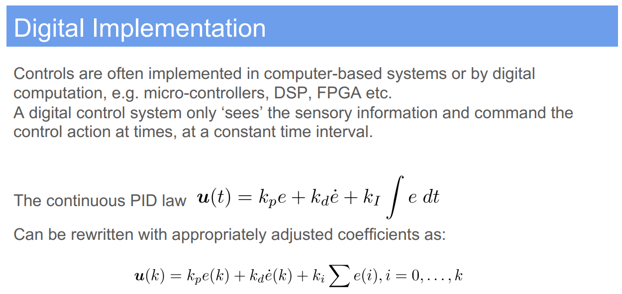
Proportional Control: $u(t) = K_p e(t)$
- Directly proportional to the error.
Integral Control: Adds integral term $K_i \int e(t) dt$
- Addresses accumulated error over time.
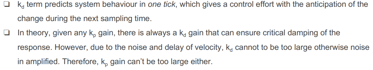
Derivative Control: Adds derivative term $K_d \frac{de(t)}{dt}$
- Predicts future error based on its rate of change.
Combined PID Control: $u(t) = K_p e(t) + K_i \int e(t) dt + K_d \frac{de(t)}{dt}$

3.5. Strengths and Limitations

Strengths:
- Simple to understand and implement.
- Effective in a variety of systems and conditions.
- Adjustable gains for system tuning.
Limitations:
- Performance can degrade in the presence of nonlinearities and disturbances.
- Requires careful tuning of parameters.
- May lead to instability if not properly configured.

3.6. Common Problems in Application

Overshoot and undershoot due to improper gain settings.
Oscillations if the derivative term is not appropriately tuned.
Steady-state error if the integral term is insufficient.

3.7. Improvement Recommendations

Implement adaptive PID control where gains adjust based on system performance.
Combine with other control strategies for handling non-linearities (e.g., feedforward control).
Use modern tuning methods like Ziegler-Nichols for optimal parameter setting.

3.8. PID Gain Tuning

There are a number of methods for tuning a PID controller to get a desired response. Below is a summary of how increasing each of the control gains affects the response:

Parameter	Rise time	Overshoot	Settling time	Steady-state error	Stability
$K_p$	Decrease	Increase	Small change	Decrease	Degrade
$K_i$	Decrease	Increase	Increase	Eliminate	Degrade
$K_d$	Minor change	Decrease	Decrease	No effect	Improve if $K_d$ small

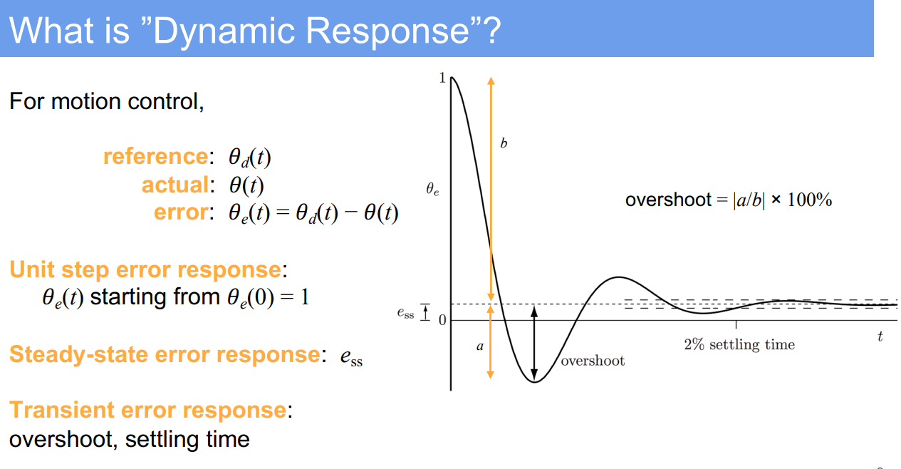
Rise Time: Rise time refers to the time it takes for the system’s response to go from a certain percentage of the steady-state value (commonly 10%) to another percentage (commonly 90%) for the first time. It’s an indicator of how quickly the system responds to a change in input.
Overshoot: Overshoot is the extent to which the system’s response exceeds its steady-state value. It’s typically measured as a percentage of the final steady-state value. High overshoot can be indicative of a system that’s too responsive and thus potentially unstable.
Settling Time: Settling time is the time taken for the system’s response to remain within a certain percentage (commonly 2% or 5%) of the steady-state value after a disturbance or a change in input. It’s a measure of how quickly the system settles into its final stable state.
Steady-State Error: Steady-state error is the difference between the system’s steady-state output and the desired output. It measures the accuracy of the system in achieving the desired output after the transient effects have died out. A well-tuned system should have a steady-state error that is as small as possible.
Stability: In control systems, stability refers to the ability of a system to converge to a steady state after a disturbance or a change in input. A stable system’s output will not diverge over time. Instability, conversely, may be indicated by oscillations that increase in amplitude over time. Stability is a fundamental requirement for any control system to be reliable and predictable in its operation.

s21174312162023

3.9. Design of PID Controllers: Discussion and Behavioral Table

The design of PID controllers is a critical step in ensuring that control systems are both responsive and stable. The balance of P, I, and D components dictates the behavior of the system’s natural frequency and damping ratio. Below is a table summarizing the general effects of increasing each PID component on the natural frequency ($\omega_n$) and damping ratio ($\zeta$):

Controller Parameter	Increase in $K_p$	Increase in $K_i$	Increase in $K_d$
Natural Frequency	Increases	Increases	Minor effect or decreases
Damping Ratio	Decreases	Increases	Increases

*Note: The exact impact on natural frequency and damping ratio can vary depending on the specific system dynamics.

In PID tuning, the aim is to achieve a desired transient response (speed of response, overshoot) and steady-state accuracy. Proportional gain $K_p$ improves the response speed but may reduce system stability, leading to oscillations. Integral gain $K_i$ eliminates steady-state error but may lead to slower response and increased overshoot. Derivative gain $K_d$ anticipates future errors, improving stability and reducing overshoot but can be sensitive to measurement noise.

The design process often involves trade-offs, and the use of tuning methods or heuristic rules can help find an optimal balance that satisfies performance criteria. Additionally, simulation tools can provide a safe environment to test and refine PID settings before applying them to the actual system.

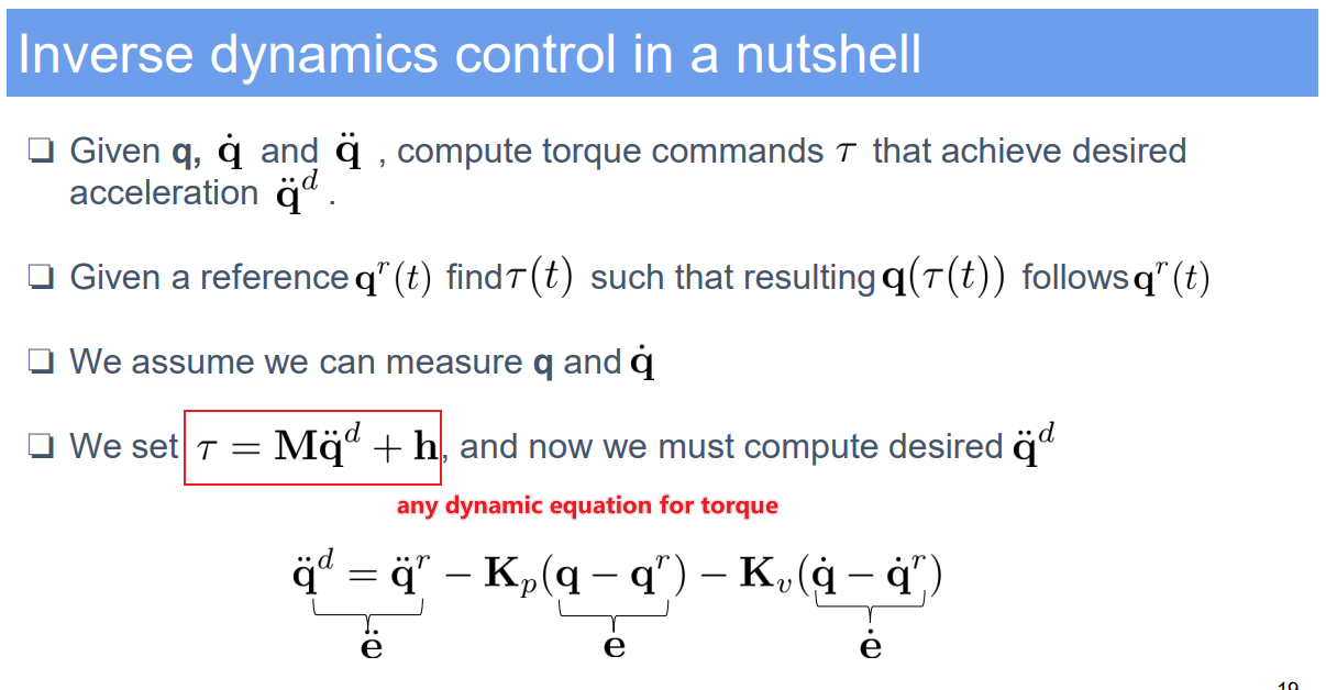
4. Inverse Dynamics Control

4.1. Demo Case Study: Robotic Arm Trajectory Tracking

Super Domain: Robotic Control Systems
Type of Method: Inverse Dynamics Control Algorithm

4.2. Problem Definition and Variables

Objective: To compute joint torques $\tau$ that achieve a desired acceleration $\ddot{q}^d$ for trajectory tracking.
Variables:
- $q$: Vector of actual joint positions.
- $\dot{q}$: Vector of actual joint velocities.
- $\ddot{q}$: Vector of actual joint accelerations.
- $q^r(t)$: Reference trajectory for joint positions at time $t$.
- $\dot{q}^r(t)$: Reference trajectory for joint velocities.
- $\ddot{q}^r(t)$: Reference trajectory for joint accelerations.
- $K_p$: Proportional gain matrix.
- $K_v$: Derivative gain matrix.
- $h$: Vector of non-linear dynamics terms including Coriolis, centrifugal, and gravitational forces.

4.3. Method Specification and Workflow

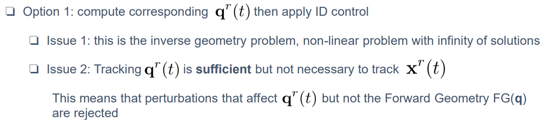
Control Law: The control torque $\tau$ is calculated to achieve the desired joint acceleration $\ddot{q}^d$ by compensating for the robot dynamics and tracking the reference trajectory.
Workflow:
1. Calculate the error in position $e = q - q^r$ and velocity $\dot{e} = \dot{q} - \dot{q}^r$.
2. Compute the desired acceleration $\ddot{q}^d$ using feedback control:
  $\ddot{q}^d = \ddot{q}^r - K_p e - K_v \dot{e}$
3. Apply the inverse dynamics formula to compute the control torques:
  $\tau = M(q) \ddot{q}^d + h$
  where $h$ includes terms for Coriolis, centrifugal, and gravitational forces.
4. Send the computed torques $\tau$ to the robot’s actuators.

4.4. Strengths and Limitations

Strengths:
- Precision in trajectory tracking due to the model-based control strategy.
- Effective compensation for the robot’s own dynamics.
Limitations:
- Highly reliant on an accurate dynamic model of the robot.
- Requires precise measurement of joint positions and velocities.

4.5. Common Problems in Application

Model inaccuracies leading to tracking errors.
Uncertainties in measuring joint velocities and accelerations.

4.6. Improvement Recommendations

Implement model identification techniques to refine the dynamic model.
Use sensor fusion to improve the accuracy of state measurements.

4.7. Inverse Dynamics Control: Discussion

Inverse dynamics control is a robust approach for commanding robotic systems to follow a desired trajectory. It involves calculating the torques that must be applied at the robot’s joints to produce the specified motion, considering the robot’s actual dynamics.

This method provides a way to design control laws that anticipate the effects of the robot’s mass, friction, and other physical properties, allowing the system to move smoothly and accurately. However, its effectiveness is highly dependent on the accuracy of the robot model used to calculate the dynamics. Any discrepancy between the model and the actual robot can result in performance degradation.

The inclusion of feedback gains $K_p$ and $K_v$ helps to correct for tracking errors and to dampen oscillations, respectively. Adjusting these gains allows for fine-tuning the control system’s responsiveness and stability.

For practitioners, this approach necessitates a deep understanding of the robot’s physical makeup and dynamics. Continuous monitoring and adjustment might be needed to maintain optimal performance, especially in changing environmental conditions or as the robot experiences wear and tear over time.

s20262212162023
s21284112162023
s21293212162023

5. Concept and definition in control

s20445712162023
s20451312162023
s20452412162023
s20453412162023
s20460812162023

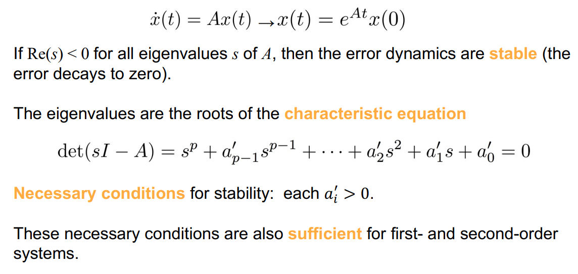
5.1. What is $Re(s)$

In the context of control theory and differential equations, $\text{Re}(s)$ refers to the real part of a complex number $s$. When discussing system stability, particularly for linear time-invariant (LTI) systems, the stability is often determined by the location of the poles of the system’s transfer function in the complex plane.

A pole is a value of $s$ (which can be complex) that makes the transfer function become unbounded. The transfer function is derived from the characteristic equation of the system’s differential equation. The characteristic equation is obtained by applying the Laplace transform to the differential equation and setting the Laplace transform of the output to zero.

For a system to be stable, all poles must have negative real parts, meaning that $\text{Re}(s) < 0$ for all eigenvalues $s$ of $A$, where $A$ is the system matrix. If $\text{Re}(s)$ is positive for any pole, the system will exhibit exponential growth in its response, leading to instability. If $\text{Re}(s)$ is zero for any pole, the system may be marginally stable or unstable depending on the multiplicity of the poles and the specific system characteristics.

Therefore, $\text{Re}(s) < 0$ is a condition for the asymptotic stability of the system, ensuring that any perturbations or errors in the system’s response will decay over time, and the system will return to its equilibrium state.

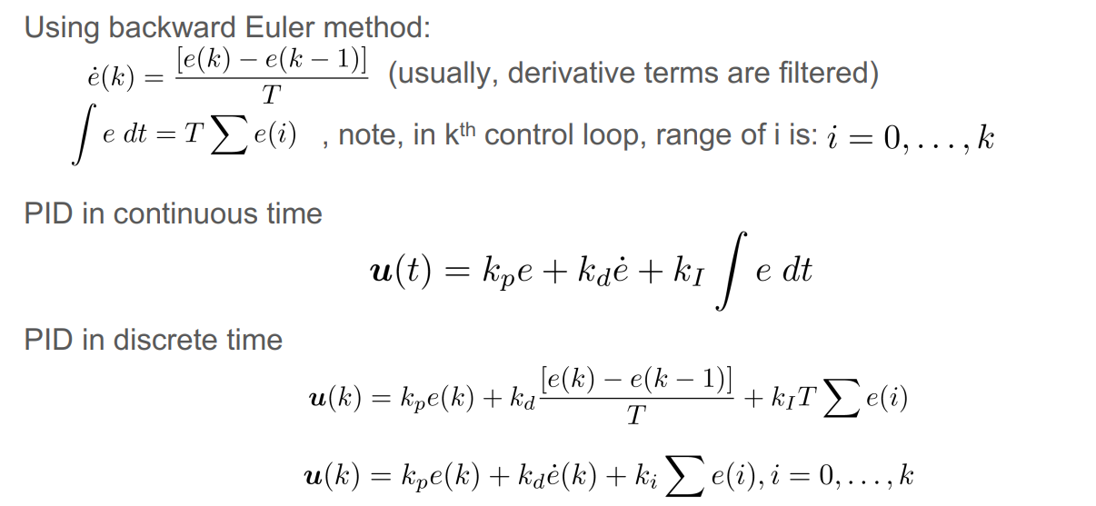
6. Digital PID control

s21193312162023
s21194212162023

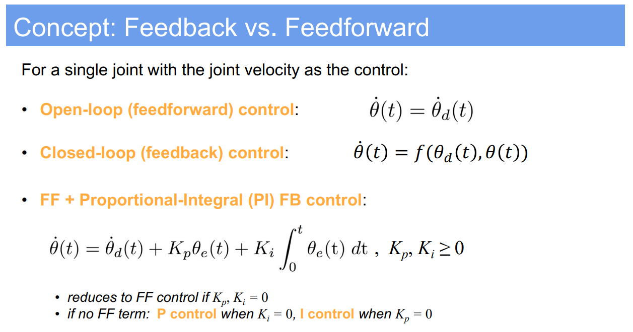
7. Feedback and feedforward control

Feedback and feedforward control are two fundamental approaches to system control in automation and robotics:

Feedforward Control (Open-loop control):
- This type of control does not use feedback to determine if its output has achieved the desired goal of the input command or process set point.
- It operates on the basis of pre-set conditions. For example, in a feedforward control system, a specific input will result in a known output without the system checking the results.
- In the context of the joint control you’ve provided, the joint velocity is set to a desired value ($\dot{\theta}_d(t)$) directly. This method assumes that the system’s behavior is predictable enough that feedback isn’t necessary.
- However, without feedback, there’s no compensation for disturbances or variations in the system’s behavior, so the actual output might differ from the expected output.
Feedback Control (Closed-loop control):
- In contrast to feedforward control, feedback control involves real-time acquisition of data related to the output or the process condition.
- The control action is based on the current state of the output and the desired output. This means that any error in the system (difference between the actual and desired output) is used to make adjustments to reach the desired goal.
- For example, $\dot{\theta}(t)$ is adjusted based on the function $f(\theta_d(t), \theta(t))$, which accounts for the actual position ($\theta(t)$) and the desired position ($\theta_d(t)$) of the joint.
Proportional-Integral (PI) Feedback Control:
- This combines both proportional control (P) and integral control (I) to adjust the controller output.
- The proportional term ($K_p$) produces an output value that is proportional to the current error value. It provides a control action to counteract the present value of the error.
- The integral term ($K_i$) is concerned with the accumulation of past error values and introduces a control action based on the sum of the errors over time, helping to eliminate steady-state errors.
- In your control equation, $\dot{\theta}(t)$ is adjusted by adding a term that accounts for the current error ($K_p \theta_e(t)$) and the integral of the error over time ($K_i \int \theta_e(t) dt$), providing a balance of immediate correction with historical error correction.

The choice between feedforward and feedback control, or a combination thereof, depends on the system requirements, the predictability of the system dynamics, and the presence of disturbances. Feedforward control is typically faster but less accurate, while feedback control can be more accurate and robust but might introduce a delay in the response.

s21210112162023

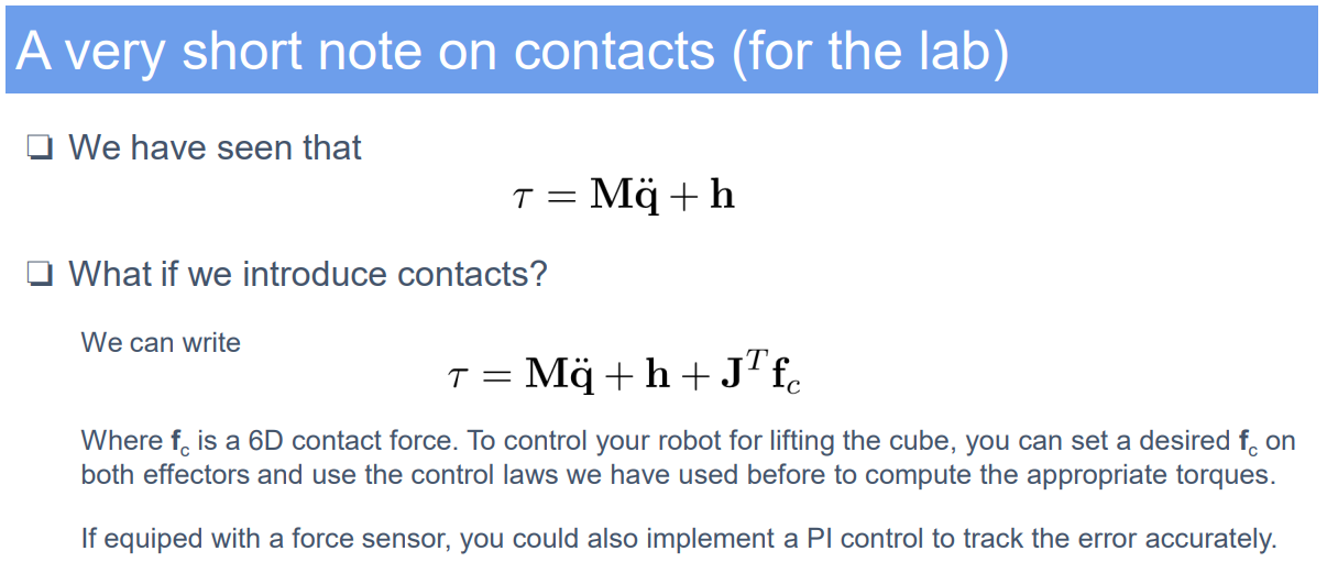
8. Apply contact force

s21313112162023

9. Optimal Control

Optimal Control is a mathematical framework aimed at finding a control policy that minimizes a certain cost function over time for a given dynamic system. The cost function typically includes terms representing the state and control effort, and may also incorporate a terminal cost evaluating the final state.

Objective:

Minimize the path cost integral plus terminal cost, formally represented as:
$\min_{X,U} \int_{0}^{T} l(x(t), u(t)) dt + l_T(x(T))$

Constraints:

The system must adhere to its dynamic model, represented by the state derivative $\dot{x}(t)$, which is a function of the current state $x(t)$ and control input $u(t)$:
$\dot{x}(t) = f(x(t), u(t))$

Variables:

$X$ and $U$ are the state and control vectors, respectively, which are functions of time $t$.
$x(t)$ represents the state vector at time $t$, mapping from real numbers to an $n$-dimensional state space.
$u(t)$ denotes the control input vector at time $t$, mapping to an $m$-dimensional control space.
The terminal time $T$ is fixed, marking the endpoint for the optimization horizon.

Discussion:
Optimal control problems are central to many engineering disciplines, particularly in robotics and automation. They provide a rigorous method for designing control systems that can perform complex tasks efficiently. However, solving these problems can be computationally challenging, especially for systems with high dimensionality or complex dynamics.

Understanding both the theory and practical application through labs is essential, as optimal control often requires a balance between theoretical knowledge and practical tuning of control parameters.

The terminal cost $l_T(x(T))$ is particularly significant as it allows incorporating goals or final conditions into the optimization process, such as reaching a target state or minimizing energy use by the terminal time $T$.

To implement an optimal control policy, one must understand the dynamic model of the system, which describes how the system evolves over time under various control inputs. This is crucial in applications like trajectory planning for autonomous vehicles, energy-efficient operation of systems, and robotic manipulator control, where the goal is to achieve desired outcomes while minimizing some notion of cost.

Reference: The University of Edinburgh, Advanced Robotics, course link
Author: YangSier (discover304.top)