ARO Additional Knowledge

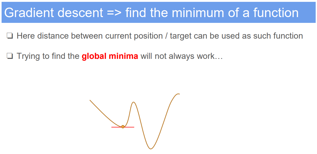
Objective: To find the optimal path for an autonomous vehicle to navigate from a starting point to a destination while minimizing a cost function.
Variables:
- $\mathbf{x}$: Vector representing the state of the vehicle (position, velocity, etc.).
- $f(\mathbf{x})$: Cost function to be minimized, e.g., distance, time, or energy consumption.

Initialization: Start with an initial guess for the state vector $\mathbf{x}$.
Gradient Calculation: Compute the gradient of the cost function, $\nabla f(\mathbf{x})$, representing the direction of steepest ascent.
Update Step: Update the state vector in the direction of the negative gradient to move towards the minimum.
- Update rule: $\mathbf{x}{new} = \mathbf{x}{old} - \alpha \nabla f(\mathbf{x}_{old})$, where $\alpha$ is the learning rate.
Iteration: Repeat the gradient calculation and update steps until convergence criteria are met (e.g., changes in cost function are below a threshold).

Strengths:
- Widely applicable to a variety of optimization problems in robotics.
- Conceptually simple and easy to implement.
- Can be adapted to different environments and cost functions.
Limitations:
- Convergence to the global minimum is not guaranteed, especially in non-convex landscapes.
- Choice of learning rate $\alpha$ is critical and can affect the speed and success of convergence.
- Computationally intensive for high-dimensional problems.

Use adaptive learning rate techniques to adjust $\alpha$ dynamically.
Implement advanced variants like stochastic gradient descent for large-scale problems.
Combine with other optimization strategies (e.g., genetic algorithms, simulated annealing) to escape local minima.

s17105112162023